Common R Portfolio
Vectorization
As a general rule of thumb, we want to avoid writing for-loops as much as possible, and instead vectorize operations to speed up our calculations. For example suppose that we want to calculate \[\sum_{i=1}^n\cos(i) \times \sin(i) \times \tan(i) - \cos(i)^2-\sin(i)^3\]
At first one could write a function similar to this:
myfunc <- function(n){
  total = 0
  for (i in 1:n){
    total = total + cos(i)*sin(i)*tan(i) - cos(i)^2 - sin(i)^3
  }
  return(total)
}
We can see see how long a function takes to run in R by using the system.time() function and look at the elapsed time:
m <- 1000000
system.time(myfunc(m))
## user system elapsed
## 0.432 0.000 0.433However this operation can be sped up by doing the same operation on each element of a vector, as follows
myfunc2 <- function(n){
  vector <- 1:n
  return(cos(vector)*sin(vector)*tan(vector) - cos(vector)^2 - sin(vector)^3)
}
then we can see that this function is much faster
system.time(myfunc2(m))## user system elapsed
## 0.184 0.004 0.188Apply family
For loops can sometimes be avoided by vectorizing our operations properly. However, this is not always the case and sometimes we need to run our operations iteratively. In R there is an alternative way of writing for loops, which uses a different syntax. We call such a family of “functions” the apply family.
In general, one should use the R apply family for clarity not for performance, as this will usually be equivalent to that of an R loop. It is important to notice that these “functions” are actually functionals. The difference is that a functional takes a function as an input and outputs a vector. As an example here is an example of a trivial functional that simply takes a vector, a function and applies such function to the vector:
myfunctional <- function(x, func){
  return(func(x))
}
Here I summarize the main members of the apply family:
apply(x, margin, fun, ..)Applies the functionfun()to the vectorxalong the dimension(s)margin. Should be used when you want to apply a function to a dimension of a matrix (or dimensions of an array).lapply(x, fun): Applies the functionfun()to the listx. This should be used when you want to applyfun()to each element of a list and obtain a list of the same length as an output.sapply(x, fun): Appliesfun()tox. Should be used likelapply()but this returns a vector. It is basicallylapply()followed byunlist().vapply(x, fun, fun_value): This works likesapply()but we can providefun_valuewhich tellsvapply()the output type and output length. This allows a speed improvement and improves consistency by matching the output withfun_value.mapply(fun, ..): Multivariate version ofsapply(). Basically, if you have a functionfun()that has \(n\) inputs, you can writemapply(fun, v1, v2, .., vn)and it will output a list where each element is the output offun(v1[i], .., vn[i]).
Side effects in the Apply Family
An important property of the apply family is that these functions have no side effects. Side effects are changes of variables in the environment you are currently working in. For example consider the following function
f <- function(x){
  x <- 1010
  return(x)
}
If we run it we get exactly what we expect 1010:
x <- 2
f(x)
## [1] 1010However, this function does not modify the value of x
x## [1] 2This means that our function f has no side effects. This is because the default behavior of R is the so called copy-on-modify which means that when we pass x to f, R does a copy of it and then when we assign x <- 1010 it assigns 1010 to such copy, leaving x as it is.
One way to modify f so that it does have a side effect is to use the superassignment operator <<- which starts from the current environment and from there works its way up to the global environemnt to try and find the variable that needs to be “superassigned”. Then, it assigns the value on the right of the superassignment operator to such variable.
f2 <- function(){
  x <<- 1010
  return(x)
}
f2()
## [1] 1010and now the value of x has been changed:
x## [1] 1010A simple example: Apply
This functional should be used with vectors having more than 1 dimension. For instance, suppose we have the following \(10\)-by-\(3\) matrix
m <- matrix(1:30, 10, 3)
m
## [,1] [,2] [,3]
## [1,] 1 11 21
## [2,] 2 12 22
## [3,] 3 13 23
## [4,] 4 14 24
## [5,] 5 15 25
## [6,] 6 16 26
## [7,] 7 17 27
## [8,] 8 18 28
## [9,] 9 19 29
## [10,] 10 20 30Then we might want to obtain a vector with \(10\) entries, each corresponding to the sum of sine of the elements of each of the rows of the matrix m. We can use apply to achive this as follows:
v1 <- apply(m, 1, function(x) sum(sin(x)))By using a for-loop we can achieve the same result
v2 <- rep(0, nrow(m))
for (row in 1:nrow(m)) {
  v2[row] <- sum(sin(m[row,]))
}
these two vectors contain the same elements
all.equal(v1, v2)## [1] TRUEThe second argument is called margin and tells apply() along which dimension we are using the function given as the third argument. For instance above we’ve used 1 which corresponds to rows. If one wanted to run the operation along the columns would use 2. For higher dimensional arrays one can use a vector of dimensions such as c(1, 2).
Map, Reduce and Filter
Map(fun, x): Applies the functionfun()to every element of the vectorx.Reduce(fun, x): Applies a function of two arguments to a vector, recursively from left to right. For instance to sum all the elements of the vector1:6we can writeReduce(function(a, b) a+b, 1:6).Filter(fun, x): Applies a function that returnsTRUEorFALSEvalues to every element of a vectorx. Basically this function is used to keep only the elements of the vectorxthat satisfy the condition encoded by the functionfun().
Parallel Computing
We want to generate points
\[y_i = \exp(1.5x_i - 1) + \epsilon_i \qquad \text{where } \epsilon_i \sim N(0, 0.64) \quad \text{for } i = 1, \ldots, 200\]
Notice that we can sample from a normal distribution using the rnorm() function. We can then generate the x_i uniformly between 0 and 1.
# Generato 200 samples from a N(0, 0.64)
e <- rnorm(n=200, mean=0, sd=0.8)
# Generate uniform x_i in [0, 1]
xunif <- runif(n=200, min=0, max=1)

phi <- function(xunif, identity=FALSE){
  xunif <- as.vector(xunif)
  # this function can transform the input into a polynomial or keep it as it is with an identity function
  if (identity==TRUE){
    return(xunif)
  } else {
    return(xunif+xunif^2+xunif^3)
  }
}
xunift <- phi(xunif)
# Calculate y_i
y <- t(exp(1.5*xunif - 1) + e)
# we need to generate the correct matrix with 1s at the end
x <- rbind(t(as.matrix(xunift)), rep(1, length(xunift)))
Now we re-write the least-squares algorithm so that it uses regularization.
reg_ls <- function(X, y, lambda=0){
  # X has to be (n features, n obs). y has to be (1, n obs)
  X <- as.matrix(X)
  y <- as.matrix(y)
  # Use solve to find the solution, rather than inverting the matrix
  A <- X%*%t(X) + diag(lambda, nrow=nrow(X), ncol=nrow(X))
  b <- X%*%t(y)
  # Notice that it defaults to lambda=0 so this function can also be used for "unregularized ls".
  return(solve(A, b))
}
Now create a utility function to evaluate the prediction, given a set of parameters
linear_ls <- function(x, w){
  # This function simply implements the linear version of f(x, w) = w^t * x
  # w will be returned as a column vector from least_squares().
  x <- as.matrix(x)
  w <- as.matrix(w)
  # Want this function to do both matrix multiplication and dot product,
  # so check for dimension and if necessary transpose
  if (dim(x)[2] != dim(w)[1]) {
    x <- t(x)
  }
  return(x%*%w)
}
At this point we want to re-implement cross-validation in a more general way. Now it uses regularized least squares and takes lambda as a parameter so that cv can now be used to find the optimal regularization parameter.
library(parallel)
library(MASS)
library(latex2exp)

cv_parallel <- function(X, y, k, lambda=0){
  # K-fold cross validation. For leave-one-out set k to num of observations.
  # X should be a (d+1)*n matrix with d = num of features, n = numb of samples.
  # y should be 1*n target vector.
  # Create a vector where errors will be stored. Length will be k
  errors <- rep(0, k)
  # First stack together X and y. y will be last row of X. Then transpose.
  xy <- t(rbind(X, y))
  # shuffle the rows
  xyshuffled <- xy[sample(nrow(xy)), ]
  # Create flags for the rows of xyshuffled to be divided into k folds
  folds <- cut(seq(1, nrow(xyshuffled)), breaks=k, labels=FALSE)
  # Go through each fold and calculate train and test stuff
  for(i in 1:k){
    # Find indeces of rows in the hold-out (test) group
    test_ind <- which(folds==i, arr.ind=TRUE)
    # Use such indeces to grab test data
    test_x <- xyshuffled[test_ind, -dim(xyshuffled)[2]]
    test_y <- xyshuffled[test_ind, dim(xyshuffled)[2]]
    # Use the remaining indeces to grab training data
    train_x <- xyshuffled[-test_ind, -dim(xyshuffled)[2]]
    train_y <- xyshuffled[-test_ind, dim(xyshuffled)[2]]
    # Now use train_x and train_y data to find the parameters. Recall that we want them
    # with num of observations as the second dimension
    w <- reg_ls(t(train_x), t(train_y), lambda=lambda)
    # Now use these parameters to find the fitted value for the current test data
    f <- linear_ls(test_x, w)
    # Now compare the function value with test_y with a suitable error function.
    e <- sum((f - test_y)^2)
    # Add error to error list
    errors[i] <- e
  }
  # Finally return the average error
  return(mean(errors))
}
Now we instantiate a set of lambdas and parallelize the operation to find the best lambda among those.
# Define a wrapper function with only one input parameter.
wrapper <- function(lambda){
  return(cv_parallel(x, y, k=ncol(y), lambda=lambda))
}
# Now create a list containing all the lambda configurations
params = 10^seq(from=-3, to=1.5, by=0.0625)
# Finally we parallelize everything
meanerrors <- mclapply(params, wrapper, mc.cores=2)
# Plot the result (requires install.packages("latex2exp"))
plot(log(params, 10), meanerrors, xlab=TeX('$\\log_{10}(\\lambda)$'), ylab=TeX('CV Error'), main=TeX('Change in CV Error due to regularization parameter'))
# Find the minimum
min_index <- which.min(unlist(meanerrors))
points(log(params, 10)[min_index], meanerrors[min_index], col='red', pch=19)
legend(x='left', legend=c("Minimum CV Error"), col=c('red'), bg='white', lwd=1)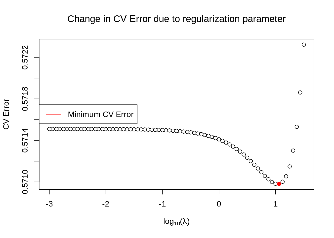
The minimum CV error is shown as a red point in the plot and corresponds to
params[min_index]## [1] 11.54782By using an optimization routine we can indeed see that this value is very close to the optimal one, which can be found like this
sol <- optimize(wrapper, params)
sol$minimum
## [1] 10.87698At this point we plot the predictive distribution. To do so, we write a wrapper function for the normal distribution, since the mean and the variance are fairly complicated functions
predictive <- function(xhat, X, y, sigmasq, lambda=sol$minimum){
  # First find the mean. This is given by the prediction by the regularized least squares. In our case, we need to find
  # W_LS-R with the current optimal value of lambda. To find it, we need to solve a system of linear equations
  X  <-  as.matrix(X)
  y <-  as.matrix(y)
  A <-  X%*%t(X) + diag(lambda, nrow=nrow(X), ncol=nrow(X))
  b <-  X%*%t(y)
  w_lsr <- solve(A, b)
  # notice xhat must be 2x1
  mean <- t(w_lsr)%*%xhat
  # Next, find the variance
  variance <- sigmasq + sigmasq*((t(xhat)%*%solve(A))%*%xhat)
  return(c(mean, variance))
}
We can plot this normal distribution as follows
# Choose a sigma squared
sigmasq <- 0.1
# Generate a new data point to predict for
xhat <- matrix(c(0.1, 1), 2, 1)
# Now find mean and variance of the predictive distribution for this data point.
meanandvar <- predictive(xhat, x, y, sigmasq)
# Use the xunif data points to plot the normal distribution with such mean and variance
xplot <- seq(-0.5, 1.5, 0.025)
plot(xplot, dnorm(xplot, mean=meanandvar[1], sd=sqrt(meanandvar[2])), main="Predictive Distribution and True Value", ylab=TeX('$p(y)$'), xlab=TeX('$y$'))
# Plot the actual value of y
abline(v=exp(1.5*0.1-1), col='red', lty=2)
legend(x='topleft', legend=c("True Value"), col=c('red'), bg='white', lwd=1, lty=2)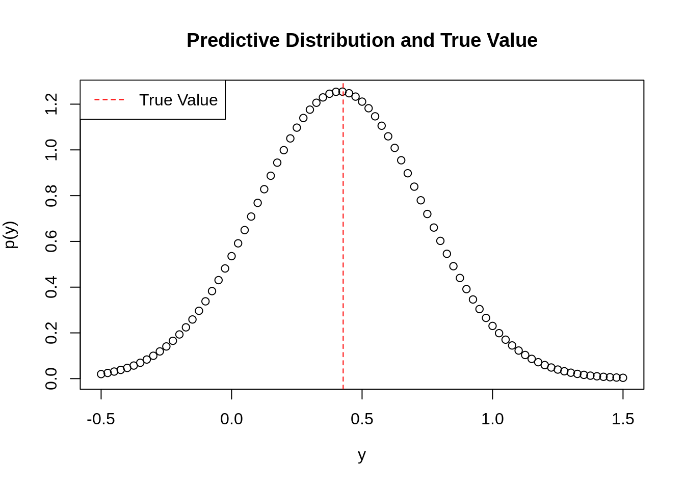
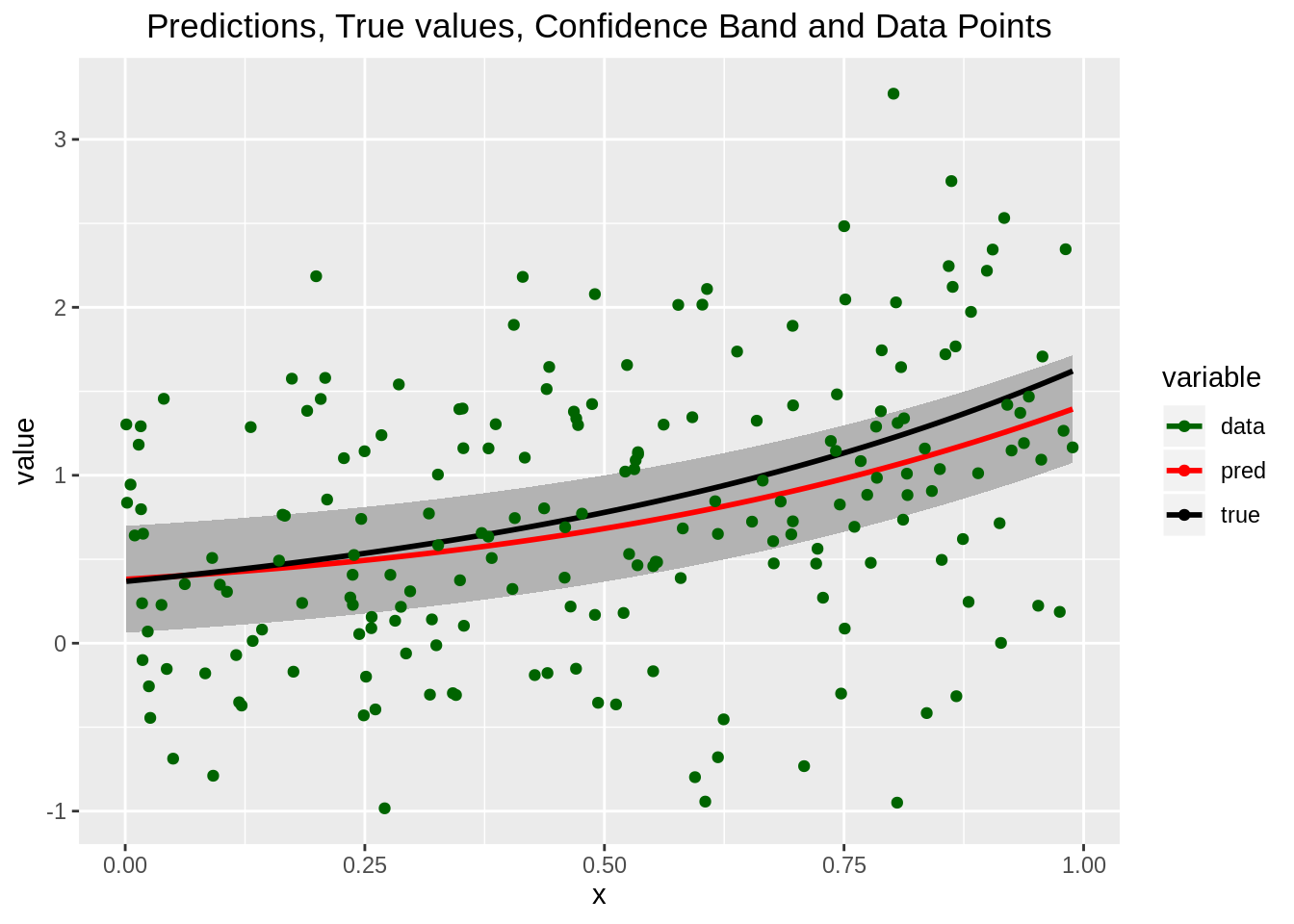
and finally we can plot the mean of the predictive distribution as \(\widehat{{\bf{x}}}\) changes.
library(ggplot2)
library(reshape2)
# wrapper function to parallelize
wrapper2 <- function(xhat){
  # recall this will be row, but need column
  xhat <- as.matrix(c(xhat, 1))
  return(predictive(xhat, x, y, sigmasq))
}
# run this parallely
result <- unlist(mclapply(xunift, wrapper2, mc.cores=2))
# Get the means and the standard deviations
means <- result[seq(1, length(result), 2)]
sds <- sqrt(result[seq(2, length(result), 2)])
# actually create a data frame with upper and lower bounds
df <- data.frame(x=xunif, m=means, lwbd=means-sds, upbd=means+sds, real=exp(1.5*xunif-1), pts=t(y))
# try melting it, might be useful later
melted <- melt(df[, -c(3, 4, 6)], id.vars="x")  # do not include upper and lower bounds, nor the points

# try plotting the melted data frame
ggplot() +
  geom_ribbon(data=df, aes(x=x, ymin=lwbd, ymax=upbd), fill="grey70") +
  geom_line(data=melted, aes(x=x, y=value, color=variable, group=variable), size=1) +
  geom_point(data=df, aes(x=x, y=pts, color='green')) +
  scale_color_manual(values=c('darkgreen', 'red', 'black'), labels=c('data', 'pred', 'true')) +
  scale_size_manual(values=c(2, 3, 3)) +
  ggtitle("Predictions, True values, Confidence Band and Data Points") +
  theme(plot.title=element_text(hjust=0.5))