
Reproducibility Portfolio
Strategies for Reproducibility
According to Lee (2019) reproducibility can be implemented by:
- Organizing files logically into modules and packages.
- Using version control software.
- Writing human-readable documentation.
Why is reproducibility important?
- If the research is reproducible, then the analysis and the methodology are clear.
- A major building block of the scientific method is the reproducibility of experiements. If independent researchers are able to reproduce our results, this will validate much coding-based research.
Replication crisis
Replication crisis refers to the difficulty or impossibility to reproduce scientific studies, which undermines their results since the reproducibility of experiments is an integral part of the scientific method. Methods to address the crisis include:
- Make our research reproducible.
- Submission of registered reports
Our research is said to be reproducible when it is possible to reproduce the same analysis and conclusions given the same raw data. Unfortunately, much of the research done up to date is irreproducible because:
- It was difficult to create code that would work seemlessly on different computer systems.
- Not all data-engineering or data cleaning steps were reported.
A registered report is a description of the methodology of the study and of the analyses before data collection. The registered report is peer-reviewed, and this guarantees that the author of the study follows a certain protocol, reducing the changes that questionable research practices are introduced.
Literate Programming
One way of making our research more reproducible is by providing human-readable code and documentation explaining the functionalities, limits and features of our code. Documentation, however, can often be neglected and quickly become outdated, which makes our code less intellegible. One way around this issue is literate programming. Literate programming combines code and documentation into the same source code, so that when code is updated, we can also update the documentation, and this should lead to a much more up-to-date documentation. One of the best ways of doing literate programming in R is to use Rmarkdown.
R Markdown
An R Markdown file is recognizable by the .rmd extension. It comprises:
A YAML header that specifies metadata such as author, title, bibliography file, and the type of output document. This section is at the top of the file and it embedded between
---before and after. For instance, the YAML file for this R Markdown is as follows
the--- title: "Reproducibility" output: html_document: toc: true toc_float: true toc_depth: 4 bibliography: bibliography.bib nocite: | @turingway ---outputfield defines what type of document we want at the end (HTML, PDF, etc),tocstands for “table of contents” and in the YAML above we’ve allowed it to show headers up to 4 levels and to “float”, i.e. to be always present at the side of the file, even when scrolling down through the document.Chunks of code and (optional) their output, such as the following:
x <- matrix(1:6, 2, 3)
dim(x)
Code chucnks are encapsulated by a pair of three consecutive backticks. After the first, curly braces are used to specify which programming language is being used and several options that go along with that code chunk, such as whether to display the output and whether the code chunk should be evaluated. For instance, to specify R code we can use## [1] 2 3{r}.Markdown.
The process to create an Rmarkdown works as follows: when we knit the document, the knitr package grabs all the code chunks, executes them and combines together the markdown text with the code and its (optional) output. Then, a free open-source document converter called pandoc transforms this combined markdown document into the desired output format, which usually is either HTML or PDF.
In the following, we’ll see several features of R markdown.
RMarkdown playground
Headers are defined by hastags. The biggest header uses only one #, and the smallest one uses six of them ######. Text can be written in italics by surrounding it with one pair of *. Using a pair of double asteriscs ** we obtain bold text. Equations can be written inline by using one pair of dollar signs \(x = z + y\) and similarly we can have an indented equation by using a pair of double dollar signs $$ \[x = z + y\]
Tables can also be constructed all in markdown
| Leftmost header | Rightmost header |
|---|---|
| lefmost cell | rightmost cell |
| bottomleft cell | bottom right cell |
Code can either be evaluated and its output shown, as demonstrated above, or the code can just appear without being evaluated byknitr using the option{r, eval=FALSE}.
x <- matrix(1:6, 2, 3)
dim(x)
To only display the output, one can use {r, echo=FALSE} to obtain
## [1] 2 3Below I’ll work through the Computing Lab of Statistical Methods 1 given in Lecture 2.
Linear Least Squares
First of all, we need to get the data from the website. Since the data is hosted as a .data file, we can use read.table() function in base R to read that file into a dataframe. Notice that the last column in the dataframe is just a boolean variable flagging whether that particular sample was used to train the model at page 38 of the corresponding book.
# Get data from the weblink
library(readr)
url <- "https://web.stanford.edu/~hastie/ElemStatLearn/datasets/prostate.data"
df <- read.table(url)[1:9]
head(df, 3)
## lcavol lweight age lbph svi lcp gleason pgg45 lpsa
## 1 -0.5798185 2.769459 50 -1.386294 0 -1.386294 6 0 -0.4307829
## 2 -0.9942523 3.319626 58 -1.386294 0 -1.386294 6 0 -0.1625189
## 3 -0.5108256 2.691243 74 -1.386294 0 -1.386294 7 20 -0.1625189We will use the columns lcavol, lweight, age, lbph, svi, lcp, gleason and pgg45 as explanatory variables, while lpsa will be our target variable. We can therefore divide the data into two dataframes:
# Recall X must have a feature in each row and an observation in each column
X <- t(as.matrix(df[1:8]))  # (d+1) * n
# We add an extra row of 1s for the bias
X <- rbind(X, rep(1, dim(X)[2]))
y <- t(as.vector(df$lpsa)) # 1 * n
Recall that in lectures the solution to linear regression least squares was given by \[{\bf{w}}_{LS} = (X X^\top)^{-1}X{\bf{y}}^\top\] where \(y=(y_1, \ldots, y_n)\in \mathbb{R}^{1\times n}\) is a row vector and \(n\) is the number of observations. The matrix \(X\in\mathbb{R}^{(d+1)\times n}\) is of the form \[ X = \begin{bmatrix} {\bf{x}}_1 & {\bf{x}}_2 & \ldots & {\bf{x}}_n\\ 1 & 1 & \ldots & 1 \end{bmatrix} \] where \({\bf{x}}_i \in \mathbb{R}^{d\times 1}\) are column vectors. Notice that \({\bf{w}}_{LS}\) can be found by solving the linear system of equations \[A{\bf{w}}_{LS} = {\bf{b}}\] where \(A = XX^\top\) and \({\bf{b}} = X{\bf{y}}^\top\). Using this trick we can write a function that returns the solution to the least squares
least_squares <- function(X, y){
  # X must have dim (d+1)*n where d = number of features, and n = number of observations
  # y must be a row vector of dim 1*n
  A <- X%*%t(X)
  b <- X%*%t(y)
  return(solve(A, b))
}
In this particular case we obtain
least_squares(X, y)## [,1]
## lcavol 0.564341280
## lweight 0.622019788
## age -0.021248185
## lbph 0.096712522
## svi 0.761673402
## lcp -0.106050939
## gleason 0.049227934
## pgg45 0.004457512
## 0.181560845Then we can evaluate \(f({\bf{x}}, {\bf{w}}_{LS})\), our fitted solution as follows
linear_ls <- function(x, w){
  # This function simply implements the linear version of f(x, w) = w^t * x
  # w will be returned as a column vector from least_squares().
  x <- as.matrix(x)
  w <- as.matrix(w)
  # Want this function to do both matrix multiplication and dot product,
  # so check for dimension and if necessary transpose
  if ((dim(x)[2] == 1) && (dim(x)[2] != dim(w)[1])) {
    x <- t(x)
  }
  return(x%*%w)
}
This function then can be used as follows
# Use 1:9 as a new observation
linear_ls(1:dim(X)[1], least_squares(X, y))
## [,1]
## [1,] 7.317851Cross Validation
The following function cv implements k-fold Cross Validation. It works by first stacking together X and y to create a new dataframe called xy that has dimension n times d+2 (it is d+2 rather than d+1 because of the extra y column.). Next, the function shuffles the rows of the dataframe using the sample() function.
At this point, we can use the cut() function to create flags that signal to which of the k groups each row of the dataframe belongs to. After this, we go through a loop where we perform least squares on all the data except the current group of rows, and we test the result exactly on that hold-out group.
cv <- function(X, y, k){
  # K-fold cross validation. For leave-one-out set k to num of observations.
  # X should be a (d+1)*n matrix with d = num of features, n = numb of samples.
  # y should be 1*n target vector.
  errors <- rep(0, k)  # errors will be stored here
  # First stack together X and y. y will be last row of X. Then transpose.
  xy <- t(rbind(X, y))
  # shuffle the rows
  xyshuffled <- xy[sample(nrow(xy)), ]
  # Create flags for the rows of xyshuffled to be divided into k folds
  folds <- cut(seq(1, nrow(xyshuffled)), breaks=k, labels=FALSE)
  for(i in 1:k){ # Go through each fold
    # Find indeces of rows in the hold-out (test) group
    test_ind <- which(folds==i, arr.ind=TRUE)
    # Use such indeces to grab test data
    test_x <- xyshuffled[test_ind, -dim(xyshuffled)[2]]
    test_y <- xyshuffled[test_ind, dim(xyshuffled)[2]]
    # Use the remaining indeces to grab training data
    train_x <- xyshuffled[-test_ind, -dim(xyshuffled)[2]]
    train_y <- xyshuffled[-test_ind, dim(xyshuffled)[2]]
    # Now use train_x and train_y data to find the parameters. Recall that we want them
    # with num of observations as the second dimension
    w <- least_squares(t(train_x), t(train_y))
    # Now use these parameters to find the fitted value for the current test data
    f <- linear_ls(test_x, w)
    # Now compare the function value with test_y with a suitable error function.
    e <- sum((f - test_y)^2)
    # Add error to error list
    errors[i] <- e
  }
  return(mean(errors)) # Finally return the average error
}
We can try this function using \(10\) fold cross validation
cv(X, y, 10)## [1] 5.261997and even leave-one-out cross validation
cv(X, y, dim(X)[2])## [1] 0.5413291Removing Features
Evaluate leave-one-out CV on the dataset where one feature has been removed each time.
errors <- rep(0, dim(X)[1]) # There's dim(X)[1] features (with bias)
for (i in 1:dim(X)[1]){     # Remove one feature at a time
  X <- X[-i, ]
  errors[i] <- cv(X, y, dim(X)[2])
}
errors
## [1] 0.7780061 0.7710748 0.8526117 0.8407295 0.8322292 0.8322292 0.8322292
## [8] 0.8322292 0.8322292The error increases because we are missing information about one of the features. We can plot the errors as follows
plot(1:length(errors), errors, xlab="Features", xaxt = "n",
     main="CV errors with feature dropping", ylab="CV errors")
labels <- names(df[1:8])
labels[9] <- "bias"
axis(1, at=1:length(errors), labels=labels)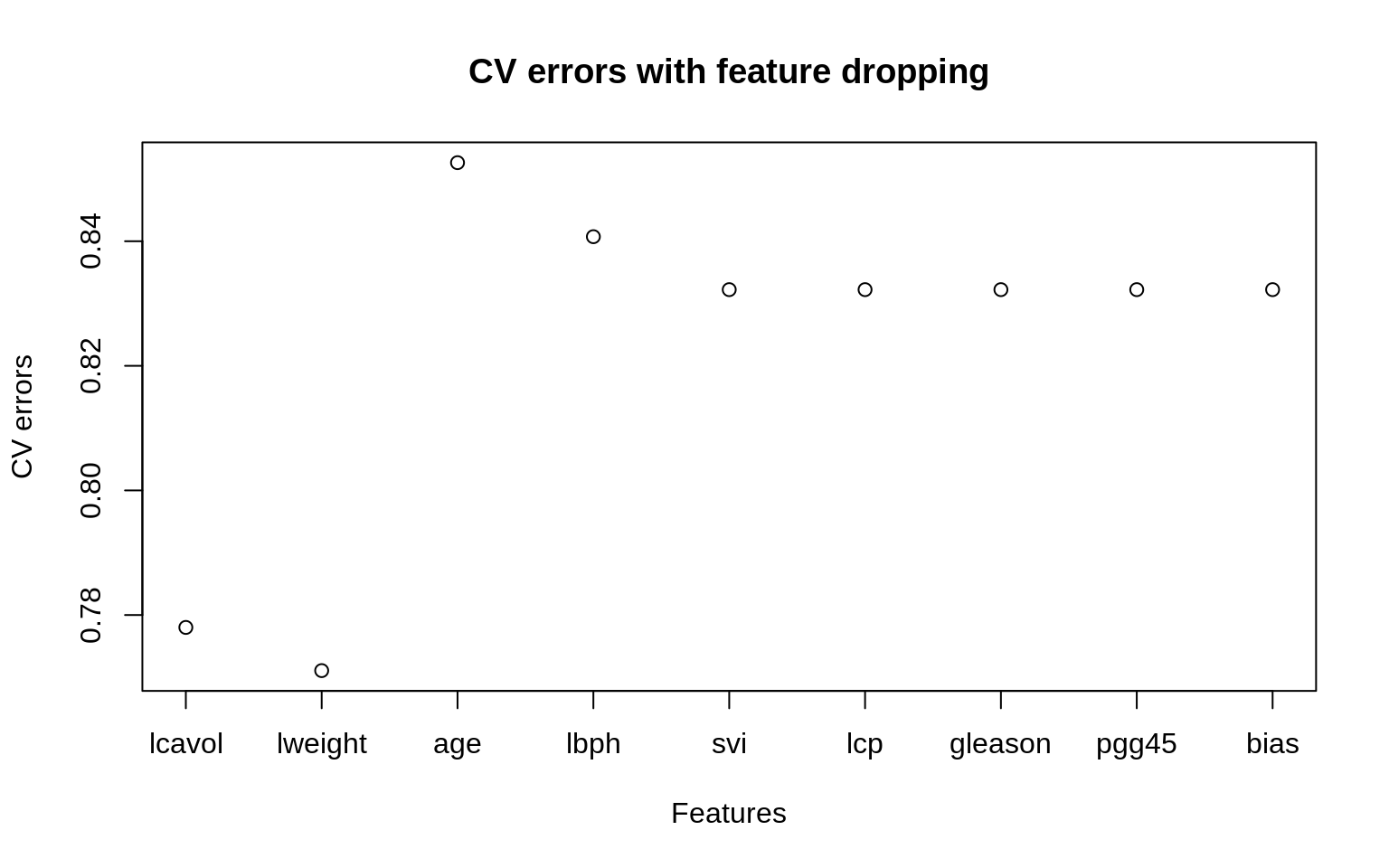
Bibliography
Lee, Anthony. 2019. “Reproducibility.” https://awllee.github.io/sc1-2019/reproducibility/.
Whitaker, Kirstie. 2019. “The Turing Way.” https://the-turing-way.netlify.com/introduction/introduction.