Random Walk Metropolis Hastings

Let’s implement a Random Walk Metropolis-Hastings algorithm with a symmetric proposal density.

rwmh <- function(start, niter, proposal, target){
  # Store accepted, rejected and all samples
  accepted <- matrix(NA, nrow=niter, dimnames=list(NULL, "accepted"))
  rejected <- matrix(NA, nrow=niter, dimnames=list(NULL, "rejected"))
  samples  <- matrix(NA, nrow=niter)
  # Set first sample to start and sample uniform random numbers for efficiency
  z <- start
  accepted[1] <- z;    rejected[1] <- z;    samples[1] <- z
  u <- runif(niter)
  # Draw candidate, calculate acceptance prob for niter-1 times
  for (i in 2:niter){
    cand <- proposal$sample(z)
    prob <- min(1, target$density(cand)/target$density(z))
    if (u[i] <= prob) {accepted[i] <- cand;    z <- cand}
    else              {rejected[i] <- cand}
    samples[i] <- z
  }
  result <- list("samples"=samples, "accepted"=accepted, "rejected"=rejected,
                 "proposal"=proposal, "target"=target)
  return(result)
}

Plotting Function

The following function takes the output of the Random-Walk Metropolis-Hastings algorithm and it produces two plots:

1. A density of the target distribution and a histogram of the samples generated by the algorithm.
2. A trace plot showing the candidates that have been proposed or accepted.

histogram_and_trace_plot <- function(out){
  # Create dataframe for target line plot and for samples histogram
  x_values  <- seq(from=out$target$range[1], to=out$target$range[2], length.out=100)
  lineplot  <- data.frame(x=x_values, y=out$target$density(x_values))
  histogram <- data.frame(x=out$samples)
  # Line plot + histogram
  bindwidth <- (out$target$range[2]-out$target$range[1]) / 50
  p <- ggplot() +
    geom_histogram(data=histogram, aes(x=x, stat(density)), binwidth = bindwidth, 
                   alpha=0.5, fill="turquoise1", color="turquoise4") +
    geom_line(data=lineplot, aes(x=x, y=y), size=1) + 
    ggtitle(paste("Target: ", out$target$name, " Proposal: ", out$proposal$name)) + 
    theme_minimal() + 
    theme(plot.title=element_text(hjust=0.5, size=15))
  # Trace plot color-coded by acceptance/rejection
  pair <- data.frame(cbind(out$accepted, out$rejected)) %>%
    transmute(sample    = coalesce(.$accepted, .$rejected), 
              flag      = as.factor((!is.na(.$accepted))), 
              iteration = row_number())
  q <- ggplot(data=pair) + 
    geom_point(aes(x=iteration, y=sample, color=flag), alpha=0.5) + 
    labs(color="Legend", size=15) + 
    scale_color_hue(labels=c("rejected", "accepted")) + 
    ggtitle("Trace Plot") + 
    theme_minimal() +
    theme(plot.title=element_text(hjust=0.5, size=15))
  grid.arrange(p, q, ncol=1)
}

Generate Functions and Data

Below we specify some density functions and some functions for sampling from specific densities.

# Targets
gamma_density <- function(x) dgamma(x, shape=2.0, scale=2.0)
beta_density <- function(x) dbeta(x, shape1=2.0, shape2=5.0)
chisq_density <- function(x) dchisq(x, df=3.0)
normal_density <- function(x) dnorm(x, mean=3)
# Proposals
normal_sample <- function(x) rnorm(1, mean=x)
beta_sample <- function(x) rbeta(1, shape1=2.0, shape2=5.0)
gamma_sample <- function(x) rgamma(1, shape=2.0, scale=2.0)
exponential_sample <- function(x) rexp(1)
# named lists
gamma <- list("density"=gamma_density, "sample"=gamma_sample, 
              "name"="Gamma", "range"=c(0.0, 20.0))
beta <- list("density"=beta_density, "sample"=beta_sample, 
             "name"="Beta", "range"=c(0.0, 1.0))
normal <- list("density"=normal_density, "sample"=normal_sample, "name"="Normal")
chisq <- list("density"=chisq_density, "sample"=NULL, 
              "name"="Chi-Squared", "range"=c(0.0, 20.0))
exponential <- list("density"=dexp, "sample"=exponential_sample, 
                    "name"="Exponential", "range"=c(0.0, 6.0))

Results

In the following plots we can see that the Random-Walk Metropolis-Hastings algorithm is indeed sampling correcly.

histogram_and_trace_plot(rwmh(0.5, 100000, normal, beta))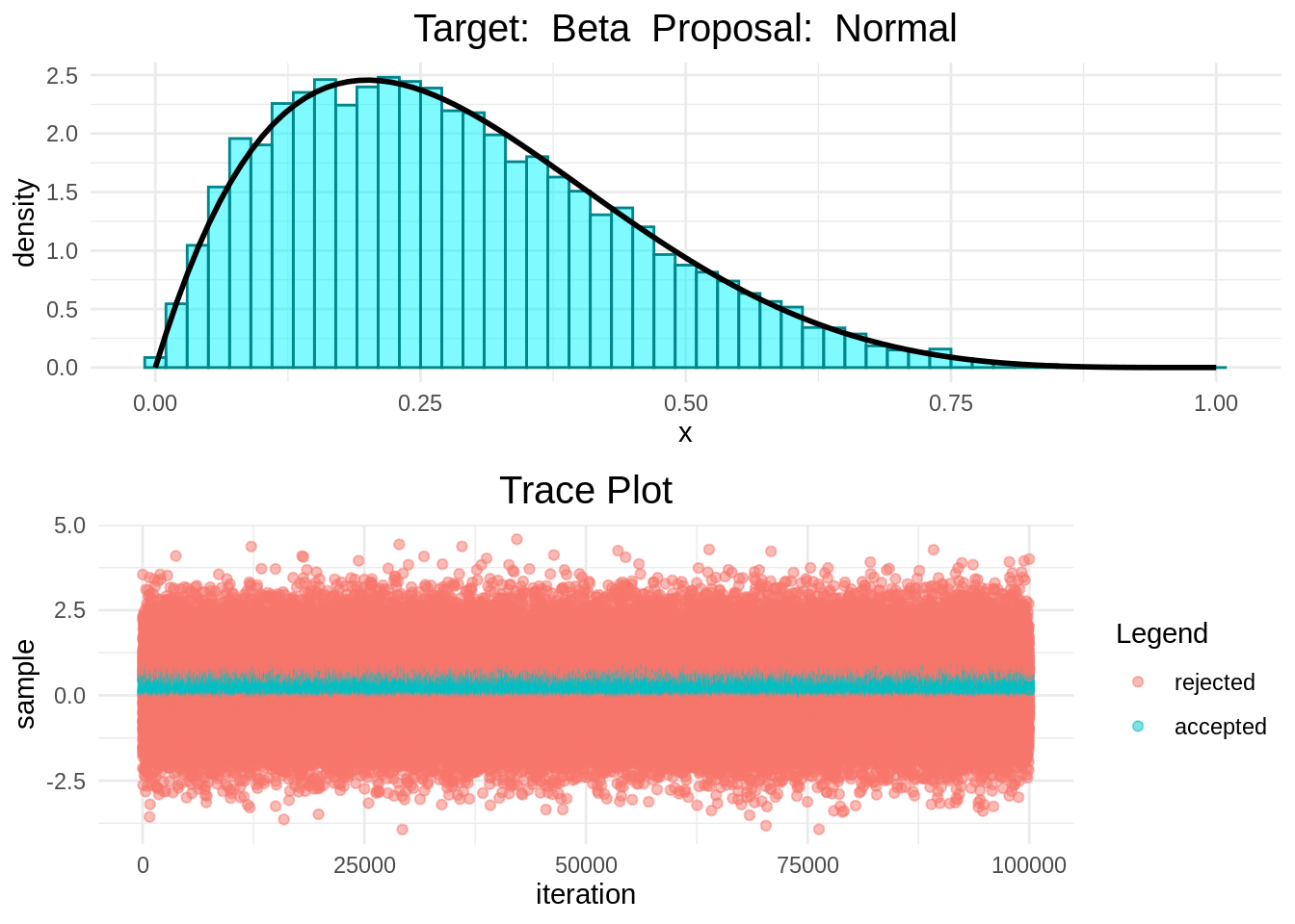

histogram_and_trace_plot(rwmh(15, 100000, normal, gamma))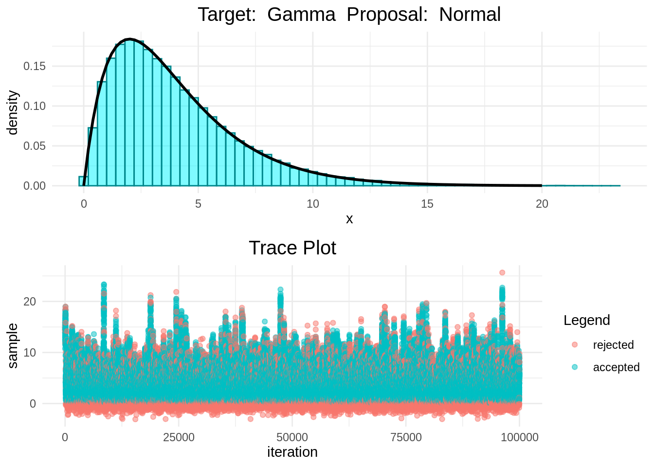

histogram_and_trace_plot(rwmh(6, 100000, normal, exponential))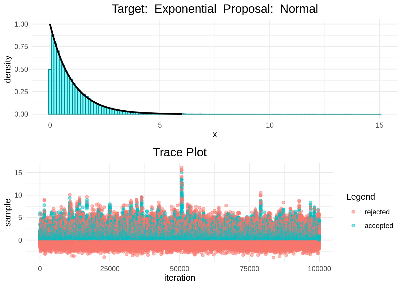

histogram_and_trace_plot(rwmh(15, 100000, normal, chisq))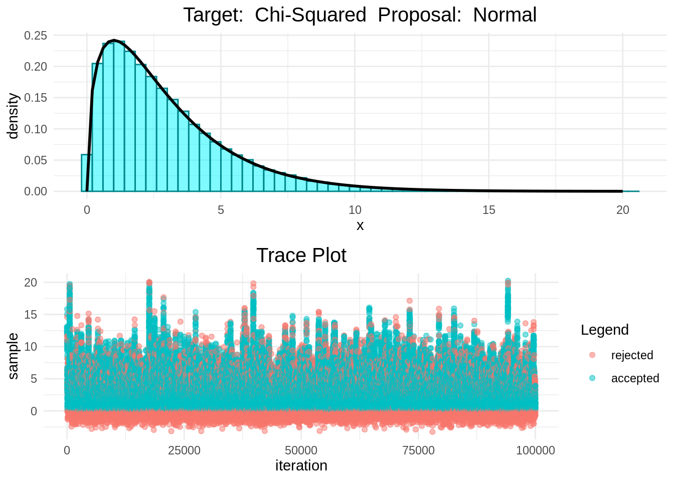

Logistic Regression Setup

Recall from the Optimization portfolio we worked with Logistic Regression. Using an isotropic Gaussian prior on our parameters the log posterior looks like this \[ \ln p(\boldsymbol{\mathbf{\beta}}\mid \boldsymbol{\mathbf{y}}) \propto -\sigma^2_{\boldsymbol{\mathbf{\beta}}}\sum_{i=1}^n\ln\left(1 + \exp((1 - 2y_i)\boldsymbol{\mathbf{x}}_i^\top\boldsymbol{\mathbf{\beta}})\right) - \frac{1}{2}\boldsymbol{\mathbf{\beta}}^\top\boldsymbol{\mathbf{\beta}} \]

Now notice that this distribution is on the \(\boldsymbol{\mathbf{\beta}}\), which means that our samples are samples of parameters.

Data Generation

Create data from two multivariate normal distributions.

n1 <- 100
n2 <- 100
m1 <- c(6, 6)
m2 <- c(-1, 1)
s1 <- matrix(c(1, 0, 0, 10), nrow=2, ncol=2)
s2 <- matrix(c(1, 0, 0, 10), nrow=2, ncol=2)
generate_binary_data <- function(n1, n2, m1, s1, m2, s2){
  # x1, x2 and y for both classes (both 0,1 and -1,1 will be created for convenience)
  class1 <- mvrnorm(n1, m1, s1)
  class2 <- mvrnorm(n2, m2, s2)
  y      <- c(rep(0, n1), rep(1, n2))   # {0 , 1}
  y2     <- c(rep(-1, n1), rep(1, n2))  # {-1, 1}
  # Generate dataframe
  data <- data.frame(rbind(class1, class2), y, y2)
  return(data)
}
# Generate reproducible data
set.seed(123)
data <- generate_binary_data(n1, n2, m1, s1, m2, s2)
X <- data %>% dplyr::select(-y, -y2) %>% as.matrix
y <- data %>% dplyr::select(y) %>% as.matrix
# need to add another colum to x to account for the bias
X <- cbind(1, X)

Multivariate Random-Walk Metropolis-Hastings Algorithm on Log Posterior

Below is a multivariate version of the Random-Walk Metropolis-Hastings algorithm defined above. This version has also been improved with the following observations:

• At the beginning samples are gonna be very much dependent on the value of start. For this reason we introduce a number of burnin iterations that are going to be thrown away. Burn-in essentially represents the “warm up” that we want to have for our algorithm.
• To remove independence we can retain every \(m^{th}\) sample. To do this, we introduce a new parameter called thinning that decides m.
• We generate all uniform samples at the start and then access them when needed.
• We use linearity of the normal distribution and thus sample niter samples from a multivariate normal distribution and then sum them to the current value.
• We also change the decision rule in a logarithm form as follows \[ \alpha=\min\left\{1, \frac{p(\text{candidate})}{p(\text{current})}\right\} = \min\left\{e^0, e^{\ln\left(p(\text{candidate}\right) - \ln\left(p(\text{current})\right)}\right\}= \min\left\{0, \ln\left(p(\text{candidate}\right) - \ln\left(p(\text{current})\right)\right\} \] so that sampling \(u\sim \mathcal{U}(0, 1)\) and the accepting if \(u\leq \alpha\) is equivalent to sampling \(u\sim\mathcal{U}(0, 1)\) and then accepting if \[ \log(u)\leq \ln\left(p(\text{candidate}\right) - \ln\left(p(\text{current})\right) \] because for \(u\in[0, 1]\) we have \(\log(u)\in(-\infty, 0]\).
• Finally, we keep track of the evaluations of the log target and recycle them. This is helpful when evaluation of the log likelihood is expensive.

rwmh_multivariate_log <- function(start, niter, logtarget, vcov, thinning, burnin){
    # Set current z to the initial point and calculate its log target to save computations
    z  <- start    # It's a column vector
    pz <- logtarget(start)
    # create vector deciding iterations where we record the samples
    store <- seq(from=(1+burnin), to=niter, by=thinning)
    # Generate matrix containing samples. Initialize with the starting value
    samples <- matrix(0, nrow=length(store), ncol=nrow(start))
    samples[1, ] <- start
    # Generate uniform random numbers in advance, to save computation. Take logarithm
    log_u <- log(runif(niter))
    # Proposal is a multivariate standard normal distribution. Generate samples and
    # later on use linearity property of Gaussian distribution
    vcov <- diag(nrow(start)) %*% vcov
    normal_shift <- mvrnorm(n=niter, mu=c(0,0,0), Sigma=vcov)
    for (i in 2:niter){
        # Sample a candidate
        candidate <- z + normal_shift[i, ]
        # calculate log target of candidate and store it in case it gets accepted
        p_candidate <- logtarget(candidate)
        # use decision rule explained in blog posts
        if (log_u[i] <= p_candidate - pz){
            # Accept!
            z  <- candidate
            pz <- p_candidate
        }
        # Finally add the sample to our matrix of samples
        if (i %in% store) samples[which(store==i), ] <- z
    }
    return(samples)
}

Define Function Proportional to Log Posterior and Run RWMH

# Up to normalization constant
log_posterior_unnormalized <- function(beta){
    log_prior      <- -0.5*sum(beta^2)
    log_likelihood <- -sum(log(1 + exp((1 - 2*y) * (X %*% beta))))
    return(log_prior + log_likelihood)
}
# To start the algorithm more efficiently, start from MAP estimate
optim_results <- optim(c(0,0,0), 
                       function(x) - log_posterior_unnormalized(x), 
                       method="BFGS", hessian=TRUE)
start <- matrix(optim_results$par)
# Use inverse of approximate hessian matrix as vcov of normal proposal
vcov  <- solve(optim_results$hessian)
# Run algorithm without burnin, with no thinning
niter <- 100000
thinning <- 1
burnin <- 0
samples <- rwmh_multivariate_log(start, niter, log_posterior_unnormalized, 
                                 vcov, thinning, burnin)

Trace Plots

samplesdf <- data.frame(samples) %>% mutate(iterations=row_number())
trace1 <- ggplot(data=samplesdf, aes(x=iterations, y=X1)) + geom_line()
trace2 <- ggplot(data=samplesdf, aes(x=iterations, y=X2)) + geom_line()
trace3 <- ggplot(data=samplesdf, aes(x=iterations, y=X3)) + geom_line()
grid.arrange(trace1, trace2, trace3, ncol=1)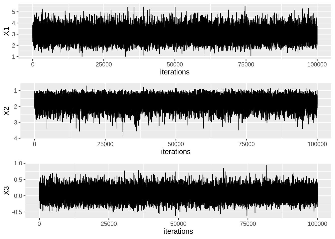

Histograms of Samples

hist1 <- ggplot(data=samplesdf, aes(x=X1, stat(density))) + 
  geom_histogram(binwidth=0.05, alpha=0.5, fill="turquoise1", color="turquoise4")
hist2 <- ggplot(data=samplesdf, aes(x=X2, stat(density))) + 
  geom_histogram(binwidth=0.05, alpha=0.5, fill="turquoise1", color="turquoise4")
hist3 <- ggplot(data=samplesdf, aes(x=X3, stat(density))) + 
  geom_histogram(binwidth=0.05, alpha=0.5, fill="turquoise1", color="turquoise4")
grid.arrange(hist1, hist2, hist3, ncol=1)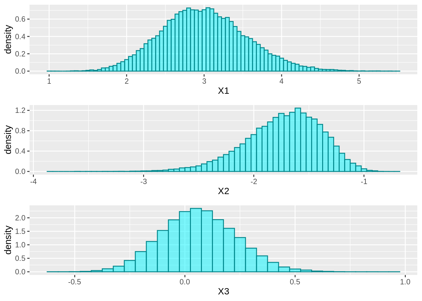

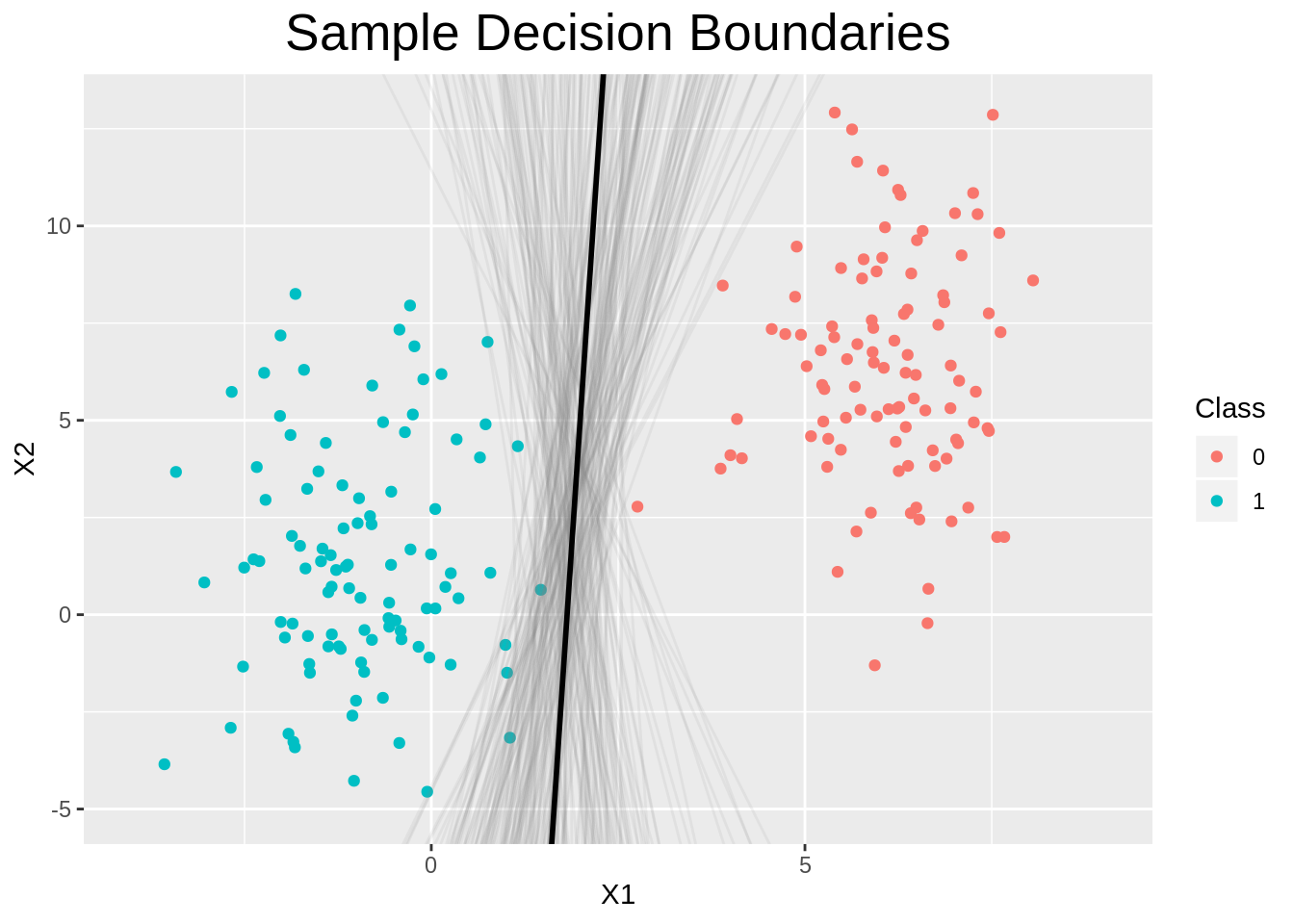
Plot decision boundary for some samples

The formula for the decision boundary is given by \[ x_2 = -\frac{\beta_1}{\beta_2}x_1 -\frac{\beta_0}{\beta_2} \] Now we use this formula to obtain the sample decision boundaries.

# Select only some samples
samples_to_select <- 200
samples_subset <- samples[sample(1:nrow(samples), samples_to_select), ]
# Calculate slope and intercept for those samples. Then calculate x2 from x1
linecoefs <- cbind(- samples_subset[, 2] / samples_subset[, 3], 
                   - samples_subset[, 1] / samples_subset[, 3])
x2_vals <- apply(linecoefs, 1, function(row) X[, 2]*row[1] + row[2])
# Store x2 values together with x1 values from X. Then melt to plot all lines 
dfsample_lines <- data.frame(x1=X[, 2], x2_vals) %>% 
  gather("key", "value", -x1)
# Create dataframe containing values for the MAP line
dfmap <- data.frame(x1=X[, 2], 
                    y=(-start[2, ]/start[3, ])*X[, 2] + (-start[1, ]/start[3, ]))
ggplot() +
  geom_point(data=data, aes(x=X1, y=X2, color=as_factor(y))) +    # Dataset scatter plot
  coord_cartesian(xlim=c(-4, 9), ylim=c(-5, 13)) + 
  geom_line(data=dfsample_lines, aes(x=x1, y=value, group=key), 
            alpha=0.1, color="grey50") +                          # Sample Lines
  geom_line(data=dfmap, aes(x=x1, y=y), color="black", size=1) +  # MAP line
  labs(color="Class", title="Sample Decision Boundaries") + 
  theme(plot.title=element_text(hjust=0.5, size=20))