Optimization Portfolio
library(MASS)
library(microbenchmark)
library(tidyverse)
Utility functions
The kernel_matrix function calculates the kernel matrix with squared exponential in a vectorized way. This function is borrowed from the profiling portfolio.
kernel_matrix <- function(X, sigmasq, Y=NULL){
  if (is.null(Y)){
    Y <- X
  }
  n <- nrow(X)
  m <- nrow(Y)
  # Find three matrices above
  Xnorm <- matrix(apply(X^2, 1, sum), n, m)
  Ynorm <- matrix(apply(Y^2, 1, sum), n, m, byrow=TRUE)
  XY <- tcrossprod(X, Y)
  return(exp(-(Xnorm - 2*XY + Ynorm) / (2*sigmasq)))
}
The function make_flags takes a y vector of length n and containing K class labels 0, 1, , K-1 and returns a matrix with n rows and K columns, where each row is a one-hot encoding for the class corresponding to that observation.
# Creates a logical one-hot encoding, assumes classes 0, .. , K-1
make_flags <- function(y){
  classes <- unique(y)
  flags <- data.frame(y=y) %>%
            mutate(rn=row_number(), value=1) %>%
            spread(y, value, fill=0) %>%
            dplyr::select(-rn) %>% as.matrix %>% as.logical %>%
            matrix(nrow=nrow(y))
  return(flags)
}
The function calc_func_per_class generate flags from the vector y and then uses each column to perform an operation on X for every element in the corresponding class.
# Calculates a function (usually mean or sd) for all classes
calc_func_per_class <- function(X, y, func){
  flags <- make_flags(y)
  return(t(apply(flags, 2, function(f) apply(X[f, ], 2, func))))
}
This is a faster version of the classic dmvnorm leveraging cholesky decomposition and computations in the log scale.
# Calculates density of a gaussian
gaussian_density <- function(x, mu, sigma, log=FALSE, precision=FALSE){
  # If precision=TRUE, we're provided with precision matrix, which is the inverse
  # of the variance-covariance matrix
  if (!precision){
    # Cholesky, L is upper triangular
    L <- chol(sigma)
    kernel <- -0.5*crossprod(forwardsolve(t(L), x - mu))
    value  <- -length(x)*log(2*pi)/2 -sum(log(diag(L))) + kernel
  } else {
    kernel <- -0.5* t(x-  mu) %*% (sigma %*% (x - mu))
    value  <- -length(x)*log(2*pi)/2 -log(det(L)) + kernel
  }
  if (!log){
    value <- exp(value)
  }
  return(value[[1]])
}
Fastest known pure-R way to compute means across dimensions.
center_matrix <- function(A){
  return(A - rep(1, nrow(A)) %*% t(colMeans(A)))
}
Binary Dataset Generation
Generate data from two multivariate gaussian distributions with similar means and same variance-covariance. Decide the number of data points for each class, the mean and the variance-covariance matrix.
n1 <- 100; m1 <- c(6, 6);  s1 <- matrix(c(1, 0, 0, 10), nrow=2, ncol=2)
n2 <- 100; m2 <- c(-1, 1); s2 <- matrix(c(1, 0, 0, 10), nrow=2, ncol=2)
Then define the data-generating function.
generate_binary_data <- function(n1, n2, m1, s1, m2, s2){
  # x1, x2 and y for both classes (both 0,1 and -1,1 will be created for convenience)
  class1 <- mvrnorm(n1, m1, s1)
  class2 <- mvrnorm(n2, m2, s2)
  y      <- c(rep(0, n1), rep(1, n2))   # {0 , 1}
  y2     <- c(rep(-1, n1), rep(1, n2))  # {-1, 1}
  # Generate dataframe
  data <- data.frame(rbind(class1, class2), y, y2)
  return(data)
}
Finally, we generate data with a random seed for reproducibility.
set.seed(123)
data <- generate_binary_data(n1, n2, m1, s1, m2, s2)
X <- data %>% dplyr::select(-y, -y2) %>% as.matrix
y <- data %>% dplyr::select(y) %>% as.matrix
Data Appearance
plot_dataset <- function(data){
  p <- ggplot(data=data, aes(x=X1, y=X2, color=as_factor(y))) +
        geom_point() +
        theme(plot.title=element_text(hjust=0.5, size=20)) +
        labs(color="Class", title="Linearly Separable Dataset")
  return(p)
}
plot_dataset(data)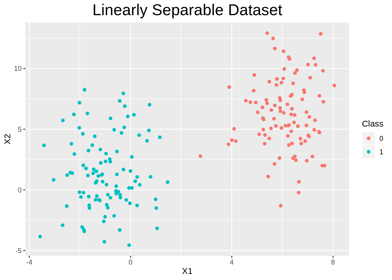
Fisher Discriminant Analysis
FDA Class
Define an S3 object performing FDA.
fda <- function(X, y){
  # Use y to create a logical one-hot encoding called `flags`
  flags <- make_flags(y)
  # Define objective function
  fda_objective <- function(w){
    mu <- mean(X %*% w)           # embedded DATASET center
    muks <- rep(0, ncol(flags))   # embedded center for class k
    swks <- rep(0, ncol(flags))   # within class scatterness
    sbks <- rep(0, ncol(flags))   # between class scatterness
    for (class in 1:ncol(flags)){
      Xk <- X[flags[, class], ]
      mk <- mean(Xk %*% w)
      muks[class] <- mk
      swks[class] <- sum(((Xk %*% w) - mk)^2)
      sbks[class] <- sum(flags[, class]) * (mk - mu)^2
    }
    # Calculate objective value
    value <- sum(sbks) / sum(swks)
    return(-value) # remember we want to maximize, but optim minimizes
  }
  # Optimize
  w_start <- matrix(1, nrow=ncol(X), ncol=1)
  sol <- optim(par=w_start, fn=fda_objective, method="BFGS")$par
  # Return object
  fda_object <- list(sol=sol, flags=flags, X=X, y=y)
  class(fda_object) <- "FDA"
  return(fda_object)
}
FDA Plot Method
plot.FDA <- function(x, y=NULL, ...){
  # Find unit vector of w and take dot product
  sol_unit <- x$sol / sqrt(sum(x$sol^2))
  dot_products <-  x$X %*% sol_unit
  if (ncol(x$X) > 2){
    # Plot on a simple horizontal line
  df <- data.frame(x1=dot_products, x2=rep(0, nrow(dot_products)), y=x$y)
  p <- ggplot(data=df) +
        geom_point(aes(x=x1, y=x2, color=as_factor(x$y)))
  } else {
    # Find embedded points in 2D
    x_emb <- dot_products %*% t(sol_unit)
    dfembed <- data.frame(x1=x_emb[, 1], x2=x_emb[, 2], y=x$y)
    # Find data mean, and mean per cluster
    datamean <- apply(x$X, 2, mean)
    datamean <- data.frame(x=datamean[1], y=datamean[2])
    meanmatrix <- calc_func_per_class(x$X, x$y, mean)
    dfclassmeans <- data.frame(meanmatrix, y=(1:nrow(meanmatrix) - 1))
    # Dataframe to plot w
    wdf <- data.frame(x=x$sol[1], y=x$sol[2], x0=c(0.0), y0=c(0.0))
    # Plot
    p <- ggplot() +
          geom_point(data=data.frame(x$X, x$y),
                     aes(x=X1, y=X2, color=as_factor(y)), alpha=0.2) +
          geom_point(data=dfclassmeans,
                     aes(x=X1, y=X2, color=as_factor(y)),
                     shape=3, size=8, show.legend=FALSE) +
          geom_point(data=datamean, aes(x=x, y=y), size=8, shape=3, color="black") +
          geom_point(data=dfembed, aes(x=x1, y=x2, color=as_factor(y))) +
          geom_segment(data=wdf,
                       aes(x=x0, y=y0, xend=x, yend=y, color="w"),
                       arrow = arrow(length=unit(0.15, "inches")),
                       color="darkred", size=1)
  }
  p +
    labs(color="Class", title="FDA-Embedded Dataset", x="X1", y="X2") +
    theme(plot.title=element_text(hjust=0.5, size=20))
}
We can now look at the results of our optimization.
fda_object <- fda(X, y)
plot(fda_object)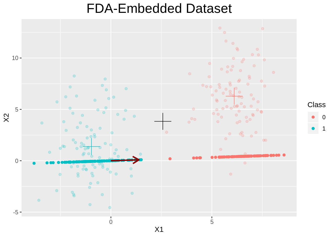
Naive Bayes
Mathematics
\[ \widehat{y} = {\arg \max}_{k\in\left\{1, \ldots, K\right\}} p(C_k) \prod_{i=1}^N p(x_i \mid C_k) \] Let’s assume each class is Gaussian distributed.
Naive Bayes Class
naive_bayes <- function(X, y){
  # For every class, find mean and variance (one class per row)
  means <- calc_func_per_class(X, y, mean)
  vars  <- calc_func_per_class(X, y, function(x) sd(x)^2)
  # Create a gaussian for each class
  nb <- list(means=means, vars=vars, X=X, y=y)
  class(nb) <- "naive_bayes"
  return(nb)
}
Predict Method
predict.naive_bayes <- function(x, xtest){
  # for every test point (row of xtest), want to calculate the density value for
  # every class, and pick the highest one.
  # Instantiate matrix of correct dimensions.
  table <- matrix(0, nrow=nrow(xtest), ncol=nrow(x$means))
  # calculate priors from data
  priors <- log(apply(make_flags(x$y), 2, function(f) length(x$y[f, ]) / length(x$y)))
  # need two for loops unfortunately
  for (r_ix in 1:nrow(xtest)){
    for (c_ix in 1:nrow(x$means)){
      # independence gives
      table[r_ix, c_ix] <- gaussian_density(
        x=matrix(as.double(xtest[r_ix, ])),
        mu=matrix(x$means[c_ix, ]),
        sigma=diag(x$vars[c_ix, ]), log=TRUE)
    }
  }
  table <- table + priors
  classes <- apply(table, 1, which.max)
  return(classes - 1)
}
Plot Method for Naive Bayes
This will plot the two classes and will predict points on a grid, to show the decision boundary.
plot.naive_bayes <- function(x, y=NULL, ngrid=75, ...){
  if (ncol(x$X) > 2) {
    print("Naive Bayes plotting for more than 2 dimensions, not implemented.")
  } else {
    # Generate a grid of points on X
    coord_range <- apply(x$X, 2, range)
    grid <- expand.grid(
      X1=seq(from=coord_range[1, 1], to=coord_range[2, 1], length=ngrid),
      X2=seq(from=coord_range[1, 2], to=coord_range[2, 2], length=ngrid)
      )
    # Use naive bayes to predict at each point of the grid
    cl <- predict(x, grid)
    dfgrid <- data.frame(grid, y=cl)
    # plot those points
    ggplot() +
      geom_point(data=dfgrid, aes(x=X1, y=X2, color=as_factor(y)), alpha=0.2, size=0.5) +
      geom_point(data=data.frame(x$X, y=x$y), aes(x=X1, y=X2, color=as_factor(y))) +
      labs(color="Class", title="Naive Bayes Decision Boundary") +
      theme(plot.title=element_text(hjust=0.5, size=20))
  }
}
plot(naive_bayes(X, y))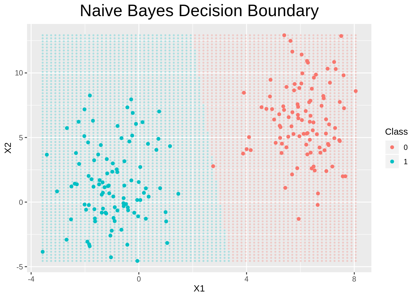
Logistic Regression
Mathematical Setting
Let \(Y_i\mid \boldsymbol{\mathbf{x}}_i \sim \text{Bernoulli}(p_i)\) with \(p_i = \sigma(\boldsymbol{\mathbf{x}}_i^\top \boldsymbol{\mathbf{\beta}})\) where \(\sigma(\cdot)\) is the sigmoid function. The joint log-likelihood is given by \[ \ln p(\boldsymbol{\mathbf{y}}\mid \boldsymbol{\mathbf{\beta}}) = \sum_{i=1}^n y_i \ln(p_i) + (1 - y_i)\ln(1 - p_i) \]
Maximum Likelihood Estimation
Maximizing the likelihood is equivalent to minimizing the negative log-likelihood. Minimizing the negative log likelihood is equivalent to solving the following optimization problem
\[ \min_{\boldsymbol{\mathbf{\beta}}}\sum_{i=1}^n\ln\left(1 + \exp((1 - 2y_i)\boldsymbol{\mathbf{x}}_i^\top\boldsymbol{\mathbf{\beta}})\right) \]
Maximum-A-Posteriori and Ridge Regularization
We can introduce an isotropic Gaussian prior on all the coefficients \(p(\boldsymbol{\mathbf{\beta}}) = N(\boldsymbol{\mathbf{0}}, \sigma_{\boldsymbol{\mathbf{\beta}}}^2 I)\). Maximizing the posterior \(p(\boldsymbol{\mathbf{\beta}}\mid \boldsymbol{\mathbf{y}})\) is equivalent to minimizing the negative log posterior \(-\ln p(\boldsymbol{\mathbf{\beta}}\mid \boldsymbol{\mathbf{y}})\) giving
\[ \min_{\boldsymbol{\mathbf{\beta}}} \sigma^2_{\boldsymbol{\mathbf{\beta}}}\sum_{i=1}^n\ln\left(1 + \exp((1 - 2y_i)\boldsymbol{\mathbf{x}}_i^\top\boldsymbol{\mathbf{\beta}})\right) + \frac{1}{2}\boldsymbol{\mathbf{\beta}}^\top\boldsymbol{\mathbf{\beta}} \] Often we don’t want to regularize the intercept. For this reason we place an isotropic Gaussian prior on \(\boldsymbol{\mathbf{\beta}}_{1:p-1}:=(\beta_1, \ldots, \beta_{p-1})\) and instead we place a uniform distribution on \(\beta_0\), which doesn’t depend on \(\beta_0\). This leads to \[ \min_{\boldsymbol{\mathbf{\beta}}} \sigma_{\boldsymbol{\mathbf{\beta}}_{1:p-1}}^2\sum_{i=1}^n\ln\left(1 + \exp((1 - 2y_i)\boldsymbol{\mathbf{x}}_i^\top\boldsymbol{\mathbf{\beta}})\right) + \frac{1}{2}\boldsymbol{\mathbf{\beta}}_{1:p-1}^\top\boldsymbol{\mathbf{\beta}}_{1:p-1} \]
Laplace Approximation
A fully-Bayesian treatment is intractable. Instead we approximate the posterior with a multivariate Gaussian distribution centered at the mode \[ q(\boldsymbol{\mathbf{\beta}}) = N\left(\boldsymbol{\mathbf{\beta}}_{\text{MAP}}, \left[-\nabla^2 \ln p(\boldsymbol{\mathbf{\beta}}_{\text{MAP}}\mid \boldsymbol{\mathbf{y}})\right]^{-1}\right) \] where one can show that the variance-covariance matrix \[ -\nabla_{\boldsymbol{\mathbf{\beta}}}^2 \ln p(\boldsymbol{\mathbf{\beta}}\mid \boldsymbol{\mathbf{y}}) = \boldsymbol{\mathbf{\Sigma}}_0^{-1} + \sum_{i=1}^n \sigma(\boldsymbol{\mathbf{x}}_i^\top \boldsymbol{\mathbf{\beta}})(1 - \sigma(\boldsymbol{\mathbf{x}}_i^\top \boldsymbol{\mathbf{\beta}})) \boldsymbol{\mathbf{x}}_i\boldsymbol{\mathbf{x}}_i^\top = \boldsymbol{\mathbf{\Sigma}}_0^{-1} + X^\top D X \] where \[ D = \begin{pmatrix} \sigma(\boldsymbol{\mathbf{x}}_1^\top\boldsymbol{\mathbf{\beta}})(1 - \sigma(\boldsymbol{\mathbf{x}}_1^\top\boldsymbol{\mathbf{\beta}})) & 0 & \ldots & 0 \\ 0 & \sigma(\boldsymbol{\mathbf{x}}_2^\top\boldsymbol{\mathbf{\beta}})(1 - \sigma(\boldsymbol{\mathbf{x}}_2^\top\boldsymbol{\mathbf{\beta}})) & \ldots & 0 \\ \vdots & \ldots & \ddots & \vdots \\ 0 & 0 & \ldots &\sigma(\boldsymbol{\mathbf{x}}_n^\top\boldsymbol{\mathbf{\beta}})(1 - \sigma(\boldsymbol{\mathbf{x}}_n^\top\boldsymbol{\mathbf{\beta}})) \end{pmatrix} \]
Gradient Ascent (MLE, No Regularization)
Updates take the form \[ \boldsymbol{\mathbf{\beta}}_{k+1} \leftarrow \boldsymbol{\mathbf{\beta}}_k + \gamma X^\top(\boldsymbol{\mathbf{y}}- \sigma(X\boldsymbol{\mathbf{\beta}}_k)) \] where the step size \(\gamma\) can either be chosen small.
Gradient Ascent (MAP, Ridge Regularization)
The update takes the form \[ \boldsymbol{\mathbf{\beta}}_{k+1}\leftarrow \boldsymbol{\mathbf{\beta}}_k + \gamma \left[\sigma_{\boldsymbol{\mathbf{\beta}}}^2X^\top(\boldsymbol{\mathbf{y}}- \sigma(X\boldsymbol{\mathbf{\beta}}_k)) - \boldsymbol{\mathbf{\beta}}_k\right] \]
Newton’s Method (MLE, No Regularization)
The iterations are as follows, where for stability one can add a learning rate \(\alpha\), which is in practice often set to \(\alpha=0.1\). \[ \boldsymbol{\mathbf{\beta}}_{k+1} \leftarrow \boldsymbol{\mathbf{\beta}}_k + \alpha(X^\top D X)^{-1} X^\top(\boldsymbol{\mathbf{y}}- \sigma(X\boldsymbol{\mathbf{\beta}}_k)) \] In practice we would solve the corresponding system for \(\boldsymbol{\mathbf{d}}\) \[ (X^\top D X)\boldsymbol{\mathbf{d}}_k = \alpha X^\top(\boldsymbol{\mathbf{y}}- \sigma(X\boldsymbol{\mathbf{\beta}}_k)) \] and then perform the update \[ \boldsymbol{\mathbf{\beta}}_{k+1}\leftarrow \boldsymbol{\mathbf{\beta}}_k + \boldsymbol{\mathbf{d}}_k \]
Newton’s Method (MAP, Ridge Regularization)
The update takes the form \[ \boldsymbol{\mathbf{\beta}}_{k+1} \leftarrow \boldsymbol{\mathbf{\beta}}_k + \alpha \left[\sigma^2_{\boldsymbol{\mathbf{\beta}}} X^\top D X + I\right]^{-1}\left(\sigma^2_{\boldsymbol{\mathbf{\beta}}} X^\top (\boldsymbol{\mathbf{y}}- \sigma(X\boldsymbol{\mathbf{\beta}}_k)) - \boldsymbol{\mathbf{\beta}}_k\right) \]
Implementations of the Optimization Methods
Below we define gradient ascent and newton’s method both for the MLE and MAP cases.
sigmoid <- function(x) 1.0 / (1.0 + exp(-x))grad_ascent <- function(beta, niter=100, gamma=0.001, cost="MLE", sigmab=1.0){
if (cost=="MLE"){
for (i in 1:niter) beta <- beta + gamma * t(X) %*% (y - sigmoid(X %*% beta))
} else if (cost=="MAP"){
for (i in 1:niter) {
beta <- beta + gamma*(sigmab^2*t(X) %*% (y - sigmoid(X %*% beta)) - beta)
}
}
return(beta)
}newton_method <- function(beta, niter=100, alpha=0.1, cost="MLE", sigmab=1.0){
# Learning rate is suggested at 0.1. For 1.0 standard Newton method is recovered
if (cost=="MLE"){
for (i in 1:niter){
D_k <- diag(drop(sigmoid(X%*%beta)*(1 - sigmoid(X%*%beta))))
d_k <- solve(t(X)%*%D_k %*% X, alpha*t(X) %*% (y - sigmoid(X %*% beta)))
beta <- beta + d_k
}
} else if (cost=="MAP"){
n <- ncol(X)
for (i in 1:niter){
D_k <- diag(drop(sigmoid(X%*%beta)*(1 - sigmoid(X%*%beta))))
d_k <- solve(
sigmab^2*t(X)%*%D_k%*%X + diag(n),
alpha*(sigmab^2*t(X)%*%(y - sigmoid(X %*% beta)) - beta)
)
beta <- beta + d_k
}
}
return(beta)
}The Logistic Regression S3 Class and Its methods
logistic_regression <- function(X, y, cost="MLE", method="BFGS", sigmab=1.0, niter=100,
                                alpha=0.1, gamma=0.001, laplace=FALSE){
  start <- matrix(0, nrow=ncol(X))
  # Define cost functions
  mle_cost <- function(beta) sum(log(1 + exp((1 - 2*y) * (X %*% beta))))
  map_cost <- function(beta) (sigmab^2)*mle_cost(beta) + 0.5*sum(beta^2)
  # Determine selected Cost Function
  if      (cost == "MLE") costfunc <- mle_cost
  else if (cost == "MAP") costfunc <- map_cost
  # Use selected method for selected cost function
  if      (method=="BFGS")   sol <- optim(par=start, fn=costfunc, method=method)$par
  else if (method=="GA")     sol <- grad_ascent(start, niter, gamma, cost, sigmab)
  else if (method=="NEWTON") sol <- newton_method(start, niter, alpha, cost, sigmab)
  # Laplace only works with MAP, not MLE
  # Can specify precision==TRUE in my builtin gaussian function
  first <- (sigmab^2)*diag(ncol(X))
  second <- t(X) %*% diag(drop(sigmoid(X %*% sol)*(1-sigmoid(X %*% sol)))) %*% X
  precision <- first + second
  # Build S3 object and return it
  lr <- list(X=X, y=y, beta=sol, cost=cost, method=method,
             prec=precision, costfunc=costfunc)
  class(lr) <- "logistic_regression"
  return(lr)
}
We provide a print method to compare results later.
print.logistic_regression <- function(x, ...){
  cat("S3 Object of Class logistic_regression.\n")
  cat("Cost Function:        ", x$cost, "\n")
  cat("Optimization Method:  ", x$method, "\n")
  cat("Solution:             ", x$beta, "\n")
}
The predict function will be useful for plotting. The sigmoid function gives the probability of being in class \(1\).
predict.logistic_regression <- function(x, xtest){
  # sigmoid gives probability of being in class 1. So will give (rounded) 1 to 1
  return(round(1.0 / (1.0 + exp(-xtest %*% x$beta))))
}
Comparing Different Optimization Implementations
Let’s run all the different algorithms with both the MLE cost function and the MAP with an isotropic gaussian as a prior. Before doing that, we need to append a column of \(1\)s to the design matrix, for the intercept term.
X <- cbind(1, X)

lr_bfgs_mle <- logistic_regression(X, y, cost="MLE", method="BFGS")
lr_bfgs_map <- logistic_regression(X, y, cost="MAP", method="BFGS")
lr_ga_mle   <- logistic_regression(X, y, cost="MLE", method="GA", niter = 1000)
lr_ga_map   <- logistic_regression(X, y, cost="MAP", method="GA", niter = 1000)
lr_nm_mle   <- logistic_regression(X, y, cost="MLE", method="NEWTON")
lr_nm_map   <- logistic_regression(X, y, cost="MAP", method="NEWTON")
In particular we can see how in general Newton is closer to BFGS than gradient ascent is. However, we can see that gradient ascent on the regularized problem seems to achieve similar results as the Newton and Quasi-Newton methods!
print(lr_bfgs_mle)## S3 Object of Class logistic_regression.
## Cost Function: MLE
## Optimization Method: BFGS
## Solution: 20.67967 -9.520793 -0.5258984print(lr_ga_mle)## S3 Object of Class logistic_regression.
## Cost Function: MLE
## Optimization Method: GA
## Solution: 3.950815 -1.976916 0.03972224print(lr_nm_mle)## S3 Object of Class logistic_regression.
## Cost Function: MLE
## Optimization Method: NEWTON
## Solution: 14.93055 -6.723051 -0.2957674print(lr_bfgs_map)## S3 Object of Class logistic_regression.
## Cost Function: MAP
## Optimization Method: BFGS
## Solution: 2.823674 -1.5538 0.05431627print(lr_ga_map)## S3 Object of Class logistic_regression.
## Cost Function: MAP
## Optimization Method: GA
## Solution: 2.782169 -1.545746 0.0572492print(lr_nm_map)## S3 Object of Class logistic_regression.
## Cost Function: MAP
## Optimization Method: NEWTON
## Solution: 2.823061 -1.552847 0.0542555Plotting
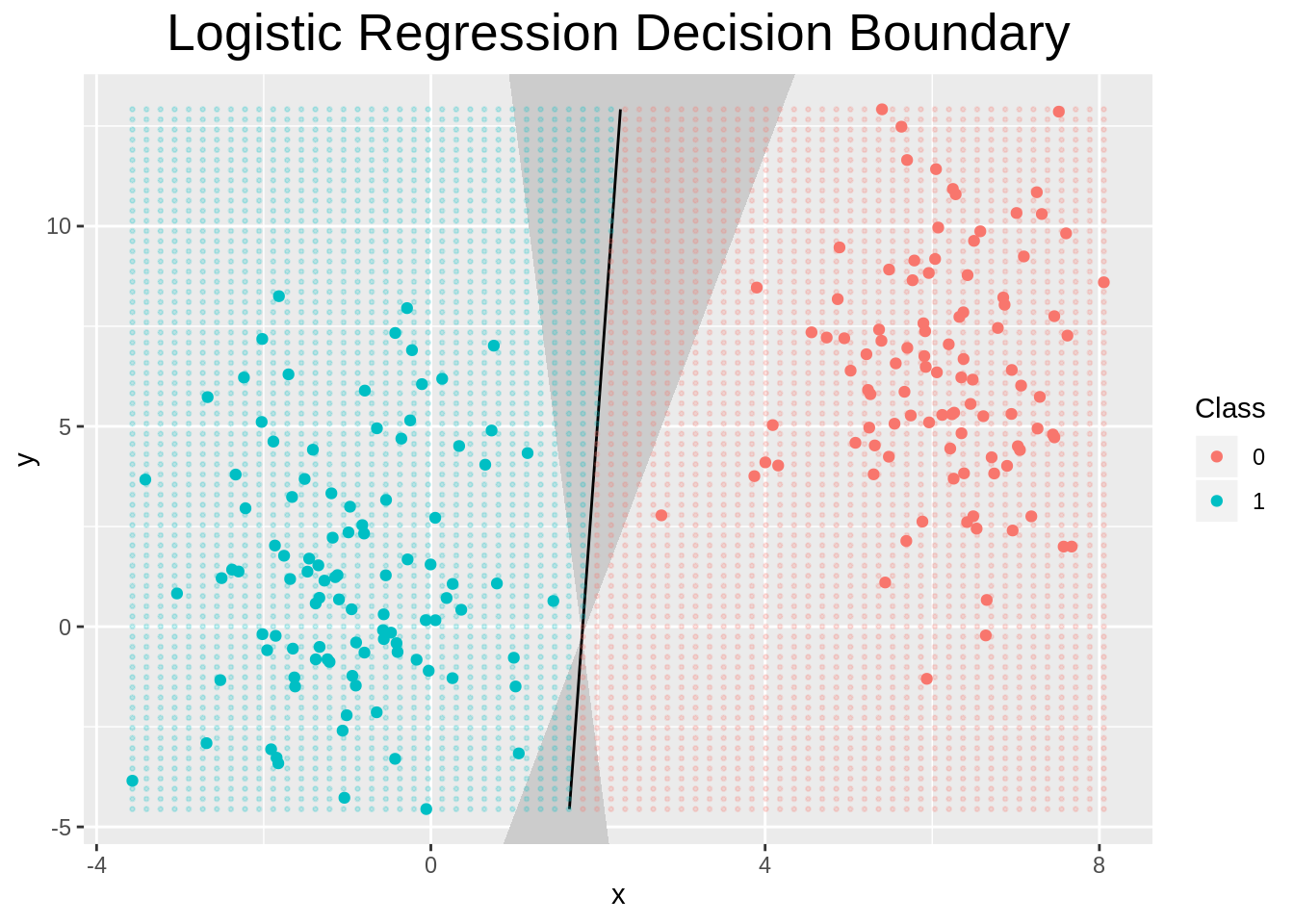
We can also specify what happens when we plot an object of class logistic_regression. In this case, we show the decision boundary and the confidence interval obtained from the Laplace Approximation to the posterior.
plot.logistic_regression <- function(x, y=NULL, ngrid=70, ...){
  # Grid to show decision boundary
  coord_range <- apply(x$X, 2, range)
  grid <- expand.grid(
      X1=seq(from=coord_range[1, 2], to=coord_range[2, 2], length=ngrid),
      X2=seq(from=coord_range[1, 3], to=coord_range[2, 3], length=ngrid)
  )
  # need to append 1 and transform to numeric, somehow it's losing it
  grid <- matrix(as.numeric(unlist(grid)), nrow=ngrid^2)
  # Predict at each point of the grid
  cl <- predict(x, cbind(1, grid))
  dfgrid <- data.frame(grid, y=cl)
  # plot those points
  p <- ggplot(data=dfgrid)
  if (!is.null(x$prec)) {
    # calculate confidence interval
    sd <- sqrt(diag(solve(x$prec)))
    beta_min <- x$beta - sd
    beta_max <- x$beta + sd
    # get range. Each column is one dimension
    ranges <- apply(x$X, 2, range)
    # understand what are the x_1 limits, from the limits of the second coordinate x_2
    x_lims <- sort((ranges[, 3] * x$beta[3] + x$beta[1]) / (-x$beta[2]))
    x1_vals <- seq(from=x_lims[1], to=x_lims[2], length.out = 200)
    x2_vals <- -(x$beta[2]/x$beta[3])*x1_vals - (x$beta[1]/x$beta[3])
    # define lines
    min_line <- function(x) -beta_min[2]*x/beta_min[3] - beta_max[1]/beta_min[3]
    max_line <- function(x) -beta_max[2]*x/beta_max[3] - beta_min[1]/beta_max[3]
    # create a poly df
    x_poly <- seq(from=ranges[1, 2], to=ranges[2, 2], length.out=500)
    dfpoly <- data.frame(x=c(x_poly,x_poly), y=c(min_line(x_poly), max_line(x_poly)))
    # same but for confidence interval
    dflaplace <- data.frame(x1=x1_vals, x2=x2_vals)
    p <- p +
      coord_cartesian(xlim=ranges[, 2], ylim=ranges[, 3])  +
      geom_polygon(data=dfpoly, aes(x=x, y=y), fill="grey80") +
      geom_line(data=dflaplace, aes(x=x1, y=x2))
  }
  p +
    geom_point(data=dfgrid, aes(x=X1, y=X2, color=as_factor(y)), alpha=0.2, size=0.5) +
    geom_point(data=data.frame(x$X, y=x$y), aes(x=X1, y=X2, color=as_factor(y))) +
    labs(color="Class", title="Logistic Regression Decision Boundary") +
    theme(plot.title=element_text(hjust=0.5, size=20))
}
We can see indeed that the laplace approximation to the posterior is more uncertain when points from either side are closer together, as one would expect.
plot(logistic_regression(X, y, cost="MAP", method="BFGS", laplace = TRUE))