
Matrices Portfolio
library(Matrix)
library(tidyverse)
library(igraph)
We work with the same dataset used for Tidyverse containing data regarding some of the top-voted kaggle kernels.
# Use `` for column names with spaces
kaggle <- "kagglekernels.csv" %>%
  read_csv(col_types = cols(
      Votes=col_double(),
      Owner=col_factor(),
      Kernel=col_factor(),
      Dataset=col_factor(),
      Output=col_character(),
      `Code Type`=col_factor(),
      Language=col_factor(),
      Comments=col_double(),
      Views=col_double(),
      Forks=col_double())
      )
kaggle # Tibbles automatically print head(tibble)
## # A tibble: 971 x 12
## Votes Owner Kernel Dataset `Version Histor… Tags Output `Code Type` Language
## <dbl> <fct> <fct> <fct> <chr> <chr> <chr> <fct> <fct>
## 1 2130 Mega… Explo… Titani… Version 8,2017-… tuto… This … Script markdown
## 2 1395 Guid… Full … Data S… Version 19,2017… tuto… This … Notebook Python
## 3 1363 Pedr… Compr… House … Version 47,2018… begi… This … Notebook Python
## 4 1316 Anis… Intro… Titani… Version 93,2018… tuto… This … Notebook Python
## 5 1078 Kaan… Data … Pokemo… Version 389,201… begi… This … Notebook Python
## 6 1003 Phil… Explo… Zillow… Version 44,2017… begi… This … Script markdown
## 7 946 Mana… Titan… Titani… Version 16,2017… tuto… This … Notebook Python
## 8 826 Omar… A Jou… Titani… Version 6,2016-… begi… This … Notebook Python
## 9 814 anok… Data … Quora … <NA> inte… This … Notebook Python
## 10 726 SRK Simpl… Zillow… Version 19,2017… eda,… This … Notebook Python
## # … with 961 more rows, and 3 more variables: Comments <dbl>, Views <dbl>,
## # Forks <dbl>Again, we can use the Tags to create a number of different new variables, each representing one Tag.
# stop here in order to have the column names
tagmatrix <- kaggle  %>%
    dplyr::select(Tags) %>%
    mutate(rn=row_number()) %>%
    separate_rows(Tags, sep="\\s*,\\s*") %>%  # RegEx comma-separated tags
    mutate(i1=1) %>%                          # Uniquely identifies rows together with rn
    mutate_all(~na_if(., "")) %>%             # remove NA generated by "<tag>,"
    pivot_wider(names_from = Tags,
                values_from = i1,
                values_fill = list(i1 = 0)) %>% # Wide format
    dplyr::select(-rn, -"NA")
tagmatrix
## # A tibble: 971 x 101
## tutorial beginner `feature engine… preprocessing eda `data cleaning`
## <dbl> <dbl> <dbl> <dbl> <dbl> <dbl>
## 1 1 1 1 0 0 0
## 2 1 0 0 1 0 0
## 3 0 1 0 0 1 1
## 4 1 0 0 0 0 0
## 5 0 1 0 0 0 0
## 6 0 1 0 0 1 0
## 7 1 0 1 0 0 0
## 8 0 1 0 0 1 0
## 9 0 0 0 0 1 0
## 10 0 0 0 0 1 0
## # … with 961 more rows, and 95 more variables: ensembling <dbl>, xgboost <dbl>,
## # `data visualization` <dbl>, `model comparison` <dbl>, `random
## # forest` <dbl>, `logistic regression` <dbl>, intermediate <dbl>, nlp <dbl>,
## # `regression analysis` <dbl>, `time series` <dbl>, `geospatial
## # analysis` <dbl>, `linear regression` <dbl>, advanced <dbl>, cnn <dbl>,
## # classification <dbl>, `neural networks` <dbl>, linguistics <dbl>, `survey
## # analysis` <dbl>, `dimensionality reduction` <dbl>, pca <dbl>, `image
## # processing` <dbl>, `deep learning` <dbl>, storytelling <dbl>,
## # databases <dbl>, bigquery <dbl>, learning <dbl>, crime <dbl>,
## # finance <dbl>, forecasting <dbl>, healthcare <dbl>, `gradient
## # boosting` <dbl>, rnn <dbl>, animation <dbl>, geography <dbl>,
## # terrorism <dbl>, `model diagnosis` <dbl>, `k-means` <dbl>, `food and
## # drink` <dbl>, `decision tree` <dbl>, animals <dbl>, `recommender
## # systems` <dbl>, `video games` <dbl>, demographics <dbl>, internet <dbl>,
## # basketball <dbl>, sports <dbl>, optimization <dbl>, `marketing
## # analytics` <dbl>, cricket <dbl>, politics <dbl>, biology <dbl>, `network
## # analysis` <dbl>, `pipeline code` <dbl>, languages <dbl>, education <dbl>,
## # `machine learning` <dbl>, gan <dbl>, regression <dbl>, business <dbl>,
## # marketing <dbl>, clustering <dbl>, `5daychallenge` <dbl>, svm <dbl>,
## # lstm <dbl>, `image data` <dbl>, `object segmentation` <dbl>,
## # statistics <dbl>, housing <dbl>, economics <dbl>, `text mining` <dbl>,
## # banking <dbl>, memory <dbl>, `association football` <dbl>, violence <dbl>,
## # `visual arts` <dbl>, history <dbl>, `bayesian statistics` <dbl>,
## # cities <dbl>, `united states` <dbl>, `occupational safety` <dbl>,
## # programming <dbl>, countries <dbl>, immigration <dbl>, `universities and
## # colleges` <dbl>, `auto racing` <dbl>, probability <dbl>, `programming
## # languages` <dbl>, plants <dbl>, firefighting <dbl>, `stochastic
## # processes` <dbl>, safety <dbl>, `outlier analysis` <dbl>, weather <dbl>,
## # `signal processing` <dbl>, `reinforcement learning` <dbl>Each column now has 1s where the Kernels were tagged with that specific tag, and 0 otherwise. Data in this form is not very useful for a graph representation. Instead, we can create an adjecency matrix having tags on columns and on rows and where the entries correspond to the number of times the pair of tags was used together in the same kernel. In order to count this metric, we can leverage the crossprod function. We also transform tagmatrix, which is a tibble, into a sparseMatrix.
tagmatrix %<>%
  as.matrix %>%
  Matrix::Matrix(sparse=TRUE) %>%
  Matrix::crossprod() %>%         # Preserves sparsity
  `diag<-`(0) %>%         # A Tag is not related with itself
  Matrix::drop0()
We can look at the sparsity pattern with the function Matrix::image() to get an idea of what this matrix looks like.
Matrix::image(tagmatrix, main="Sparsity Patter of Tag Pairings")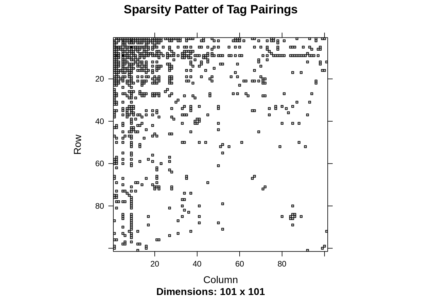
Alternatively, we can look at the percentage of sparsity.
nnzero(tagmatrix) / length(tagmatrix)## [1] 0.08214881We now proceed to use the igraph package to plot a network using tagmatrix as a weighted adjecency matrix. Since the matrix is very large, we restrict ourselves to the most “social” tags, i.e. tags that have been paired with other tags more than a given number of times, in this case 5. To do this, we set those values to zero and then drop the corresponding column and rows (since tagmatrix is symmetric).
# set values below a threshold to 0
tagmatrix[tagmatrix<=5] <- 0
# drop empty rows and columns for graphing purposes
flag <- apply(tagmatrix, 1, function(x) any(x != 0))
tagmatrix <- tagmatrix[flag, flag]
# value corresponds to how "social" those tags are
graph <- graph_from_adjacency_matrix(tagmatrix, weighted = TRUE)
We first choose to plot the network using a standard circle layout.
plot(graph, layout=layout_in_circle(graph), vertex.label.cex=1.0,
     edge.arrow.size=1.0, vertex.label.color="black", vertex.size=24)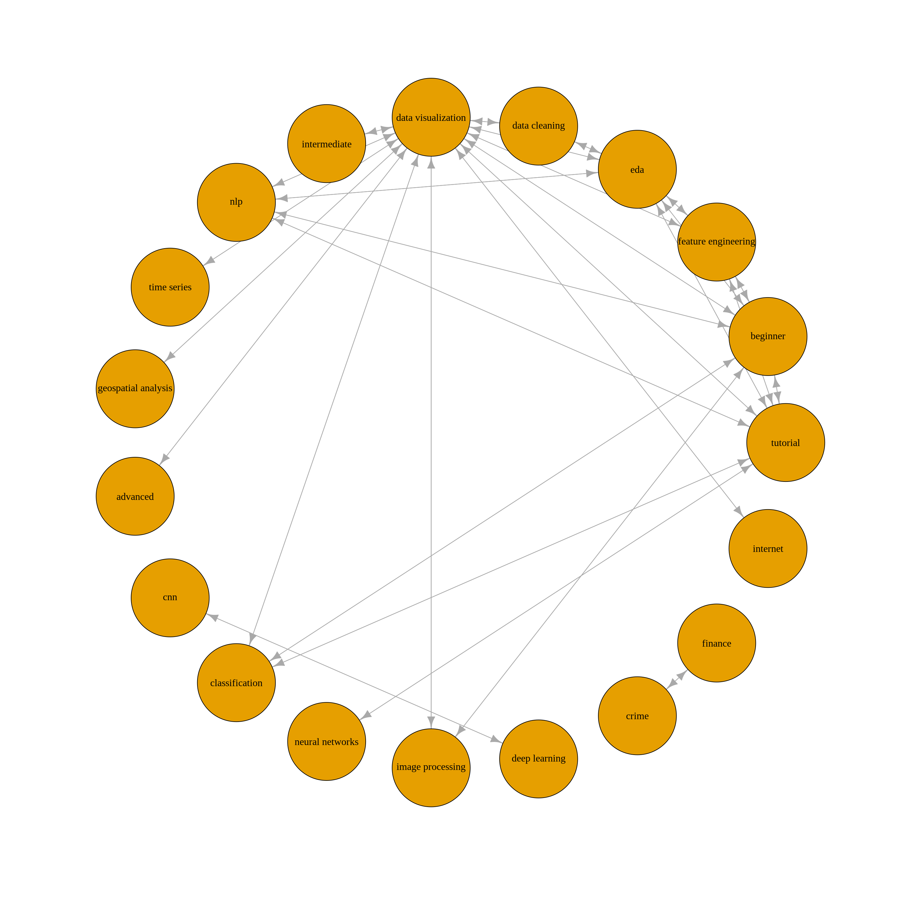
While at first this graph looks insightful, it’s hard to see some structure. Rather, we can specify a layout by choosing ourselves the coordinates of each node. After some trail and error, it’s possible to come up with a layout similar to this one.
# graph
layout <- matrix(c(0, 1, 1, 0, -1, 2, 3, -1, 3, 4, 4, 1, 1, -1, 2, 0, 3, 4, 4,
                   0, 1, 2, 2,  2, 1, 2,  1, 0, 0, 2, 3, 0,  0, 0, 3, 3, 3, 1), nrow=19, ncol=2)
plot(graph, layout=layout, vertex.label.cex=1.0, edge.arrow.size=1.0,
     vertex.label.color="black", vertex.size=24)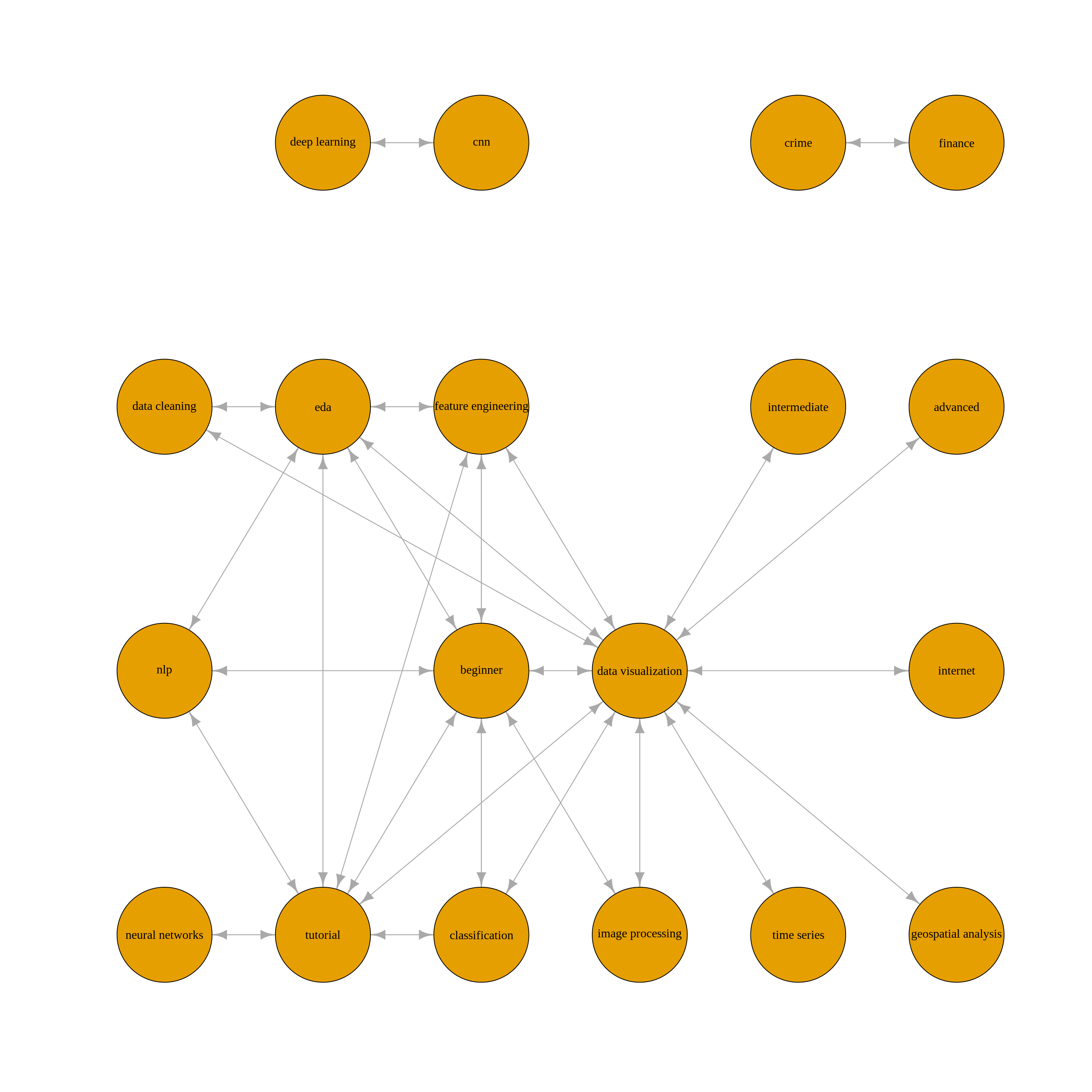
We can see a few important features. First of all it looks like there are three main clusters. One is about deep learning, one is about finance and crime data and the other cluster gathers together most other variables. In this latter cluster, we can see that data visualization dominates.