
Profiling Portfolio
Implementations
Data Generation and Problem Settings
Import the necessary packages. The library provfis is a stochastic profiler and can be used to profile our code.
library(profvis)
library(tidyverse)
library(MASS)
library(microbenchmark)
First, let’s decide some parameters and settings such as the amount of training and testing data.
# Number of data points for plotting & Bandwidth squared of the RBF kernel
ntest <- 500
# Characteristic Length-scale for kernel
sigmasq <- 1.0
# Number of training points, standard deviation of additive noise
ntrain <- 10
sigma_n <- 0.5
# Define number of samples for prior gp mvn and posterior gp mvn to take
nprior_samples <- 5
npost_samples <- 5
Define some helper functions. In particular, the kernel function is a squared exponential. The bandwidth is computed as the median of all pairwise distances. We also define a matrix that applies the squared exponential to rows of two matrices, i.e. it computes the kernel matrix \(K(X, Y)\). for two matrices \(X\) and \(Y\). Finally, we also have a regression function which represents the true structure of the data. This is just a quintic polynomial for simplicity, but can be replaced by more complicated functions.
squared_exponential <- function(x, c, sigmasq){
  return(exp(-0.5*sum((x - c)^2) / sigmasq))
}
kernel_matrix <- function(X, Xstar, sigmasq){
  # compute the kernel matrix
  K <- apply(
    X=Xstar,
    MARGIN=1,
    FUN=function(xstar_row) apply(
      X=X,
      MARGIN=1,
      FUN=squared_exponential,
      xstar_row,
      sigmasq
      )
    )
  return(K)
}
regression_function <- function(x){
    val <- (x+5)*(x+2)*(x)*(x-4)*(x-3)/10 + 2
  return(val)
}
Now let’s actually generate some data
set.seed(12345)
# training data
xtrain <- matrix(runif(ntrain, min=-5, max=5))
ytrain <- regression_function(xtrain) + matrix(rnorm(ntrain, sd=sigma_n))
# testing data
xtest <- matrix(seq(-5,5, len=ntest))
Naive Vectorized Implementation
The first implementation that we look at is naive in the sense that it basically blindly copies the operations. This means that we invert \(K + \sigma_n^2 I\) directly.
source("gp_naive.R", keep.source = TRUE)
profvis(result <- gp_naive(xtrain, ytrain, xtest, sigma_n, sigmasq))
Online Non-Vectorized Cholesky Implementation
This implementation can also be used online. It is recommended in the “Gaussian Processes for Machine Learning” book.
source("gp_online.R", keep.source = TRUE)
profvis(result_online <- gp_online(xtrain, ytrain, xtest, sigma_n, sigmasq))
Online Vectorized-Kernel Cholesky Implementation
We can see that most of the time is spent computing the kernel matrix. We can therefore find a faster way to compute it as follows
kernel_matrix_vectorized <- function(X, sigmasq, Y=NULL){
  if (is.null(Y)){
    Y <- X
  }
  n <- nrow(X)
  m <- nrow(Y)
  # Find three matrices above
  Xnorm <- matrix(apply(X^2, 1, sum), n, m)
  Ynorm <- matrix(apply(Y^2, 1, sum), n, m, byrow=TRUE)
  XY <- tcrossprod(X, Y)
  return(exp(-(Xnorm - 2*XY + Ynorm) / (2*sigmasq)))
}
using this, we get
source("gp_online_vect.R", keep.source = TRUE)
profvis(gp_online_vect(xtrain, ytrain, xtest, sigma_n, sigmasq))
We can see that this implementation uses much less memory and it’s much faster.
Completely vectorized implementation
We can combine these ideas to obtain a much faster implementation.
source("gp_completely_vectorized.R", keep.source = TRUE)
profvis(gp_completely_vectorized(xtrain, ytrain, xtest, sigma_n, sigmasq), interval=0.005)
Visualizations
Before seeing training data
Before seeing the training data we only have the test data. The Gaussian Process will therefore predict random (smooth) functions with mean zero.
Kss <- kernel_matrix_vectorized(xtest, sigmasq)
# Sample nprior_samples Multivariate Normals with mean zero and variance-covariance
# being the kernel matrix
data.frame(x=xtest, t(mvrnorm(nprior_samples, rep(0, length=ntest), Kss))) %>%
  setNames(c("x", sprintf("Sample %s", 1:nprior_samples))) %>%
  gather("MVN Samples", "Value", -x) %>%
  ggplot(aes(x=x, y=Value)) +
    # Because diag(Kss) are all 1s. We use mean +\- 2*standard deviation
    geom_rect(xmin=-Inf, xmax=Inf, ymin=-2, ymax=2, fill="grey80") +
    geom_line(aes(color=`MVN Samples`)) +
    geom_abline(slope=0.0, intercept=0.0, lty=2) +
    scale_y_continuous(lim=c(-3, 3)) +
    labs(title=paste(nprior_samples, "MVN Samples before seeing the data")) +
    theme(plot.title=element_text(hjust=0.5))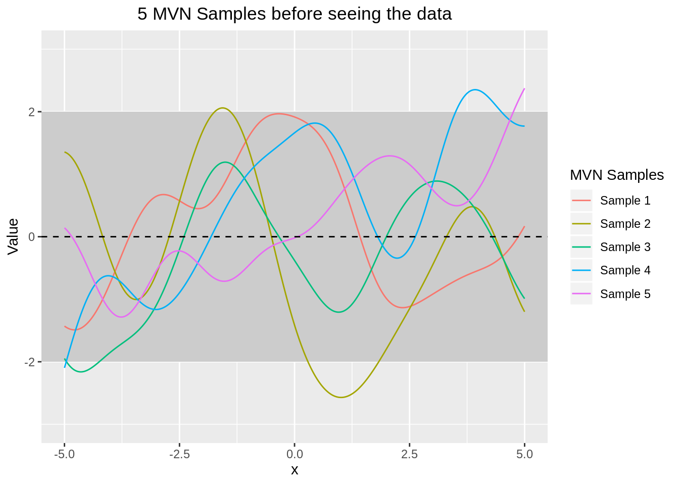
After seeing training data
We only need to find the predicted mean and the predicted variance.
# Get predicitons. To predict noisy data just add sigma_n^2*diag(ncol(xtest))
# to the covariance matrix as implemented in the script
results <- gp_completely_vectorized(xtrain, ytrain, xtest, sigma_n, sigmasq)

gpmean <- results[[1]]
gpvcov <- results[[2]]
# for plotting
dftrain = data.frame(xtrain=xtrain, ytrain=ytrain)
# Plot
data.frame(x=xtest, t(mvrnorm(npost_samples, gpmean, gpvcov))) %>%
  setNames(c("x", sprintf("Sample %s", 1:npost_samples))) %>%
  mutate(ymin=gpmean-2*sqrt(diag(gpvcov)), ymax=gpmean+2*sqrt(diag(gpvcov)),
         gpmean=gpmean, ytrue=regression_function(xtest)) %>%
  gather("MVN Samples", "Value", -x, -ymin, -ymax, -gpmean, -ytrue) %>%
  ggplot(aes(x=x, y=Value)) +
    geom_ribbon(aes(ymin=ymin, ymax=ymax), fill="grey80") +
    geom_line(aes(color=`MVN Samples`)) +
    geom_line(aes(y=gpmean), size=1) +
    geom_line(aes(y=ytrue), color="darkred", lty=2) +
    geom_point(data=dftrain, aes(x=xtrain, y=ytrain), color="red") +
    ggtitle(paste(npost_samples, "MVN Samples after seeing", ntrain, "data points")) +
    theme(plot.title=element_text(hjust=0.5))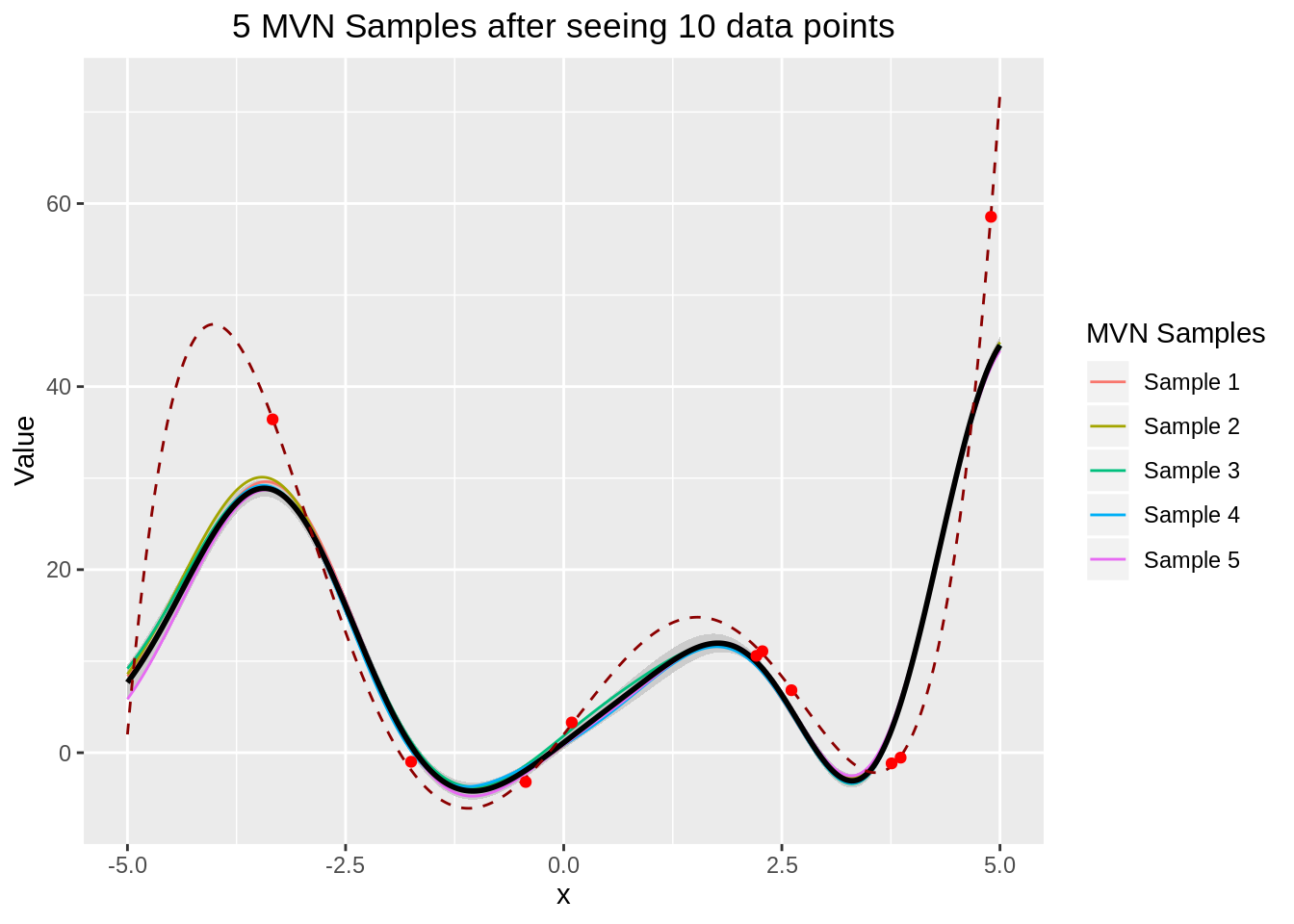
Note on Vectorized Kernel Matrix
One might wonder why in the function kernel_matrix_vectorized() we fill the matrix Ynorm by row. Afterall R works with column-major storage so this should be inefficient. One can compare filling in a matrix by row versus filling it by column and then taking the transpose in different cases:
- Number of rows < Number of columns
nrows <- 100
ncols <- 2000
microbenchmark(
  rowwise=matrix(0, nrows, ncols, byrow=TRUE),
  transpose=t(matrix(0, nrows, ncols))
  )
## Unit: microseconds
## expr min lq mean median uq max neval
## rowwise 321.202 343.0085 648.0742 360.0345 697.1185 5734.401 100
## transpose 534.310 569.7350 950.3921 608.9455 1233.3545 3354.230 100- Number of rows = Number of columns
nrows <- 2000
ncols <- 2000
microbenchmark(
  rowwise=matrix(0, nrows, ncols, byrow=TRUE),
  transpose=t(matrix(0, nrows, ncols))
  )
## Unit: milliseconds
## expr min lq mean median uq max neval
## rowwise 16.69890 24.08596 26.52232 24.48049 28.26676 91.81093 100
## transpose 23.32213 29.73081 38.70225 36.65087 41.26867 96.43356 100- Number of rows > Number of columns
nrows <- 2000
ncols <- 100
microbenchmark(
  rowwise=matrix(0, nrows, ncols, byrow=TRUE),
  transpose=t(matrix(0, nrows, ncols))
  )
## Unit: microseconds
## expr min lq mean median uq max neval
## rowwise 378.090 383.898 470.1237 392.2410 398.4715 2512.430 100
## transpose 564.521 579.105 688.0039 593.8405 621.8380 2687.371 100Generally, byrow=TRUE is faster.