
Functional Programming Portfolio
Mathematical Set Up
Suppose we have a training matrix \(X\) with \(n\) observations and \(d\) features \[ X = \begin{pmatrix} x_{11} & x_{12} & \ldots & x_{1d}\\ x_{21} & x_{22} & \ldots & x_{2d} \\ \vdots & \vdots & \ddots & \vdots \\ x_{n1} & x_{n2} & \ldots & x_{nd} \end{pmatrix} =\begin{pmatrix} {\bf{x}}_1^\top \\ {\bf{x}}_2^\top \\ \vdots \\ {\bf{x}}_n^\top \end{pmatrix} \in\mathbb{R}^{n\times d} \] and that we want to do a feature transform of this data using the Radial Basis Function. To do this, we
- choose \(b\) rows of \(X\) and we call them centroids \[ {\bf{x}}^{(1)}, \ldots, {\bf{x}}^{(b)} \]
- calculate using some heuristic a bandwidth parameter \(\sigma^2\)
And then, for every centroid we define a radial basis function as follows
\[
\phi^{(i)}({\bf{x}}):=\exp\left(- \frac{\parallel{\bf{x}} - {\bf{x}}^{(i)}\parallel^2}{\sigma^2}\right) \qquad \forall i\in\{1, \ldots, b\} \quad \text{for } {\bf{x}}\in\mathbb{R}^{d}
\]
We can therefore obtain a transformed data matrix as
\[
\Phi:=\begin{pmatrix}
1 & \phi^{(1)}({\bf{x}}_1) & \phi^{(2)}({\bf{x}}_1) & \cdots & \phi^{(b)}({\bf{x}}_1) \\
1 & \phi^{(1)}({\bf{x}}_2) & \phi^{(2)}({\bf{x}}_2) & \cdots & \phi^{(b)}({\bf{x}}_2) \\
\vdots & \vdots & \vdots & \ddots & \vdots \\
1 & \phi^{(1)}({\bf{x}}_n) & \phi^{(2)}({\bf{x}}_n) & \cdots & \phi^{(b)}({\bf{x}}_n)
\end{pmatrix} \in\mathbb{R}^{n\times (b+1)}
\]
Then we fit a regularized linear model so that optimal parameters are given by
\[
{\bf{w}}:=(\Phi^\top\Phi + \lambda I_n)^{-1}\Phi^\top{\bf{y}}
\]
These parameters are usually found by solving the associated system of linear equations for \({\bf{w}}\)
\[
(\Phi^\top\Phi + \lambda I_n) {\bf{w}} = \Phi^\top {\bf{y}}
\]
This will be one of the strategies that we’ll see below. However, we are required to apply regularization with a very small regularization parameter \(\lambda\). This hints at the fact that maybe we can simply set \(\lambda=0\) and then find \({\bf{w}}\) simply by finding the pseudoinverse of \(\Phi\)
\[
(\Phi^\top\Phi)^{-1}\Phi^\top
\]
and then multiply this by \({\bf{y}}\) on the left. This approach looks more stable and can be implemented by setting pseudoinverse=TRUE in the function make_predictor defined in this document.
Parameters
In the following code chunk you can set up \(n\) the number of training observations, \(d\) the dimensionality of the input (i.e. the number of features), \(\lambda\) the regularization coefficient, \(m\) the number of testing observations, and \(b\) dimensionality of the data after the feature transform, which in this case corresponds to the number of centroids.
n <-  1000
d <-  2
lambda <-  0.00001
m <-  200
b <-  50
Training and Testing Sets
We work with synthetic data sets. For simplicity, we will generate \(X\) uniformly in an interval (which in this case is \([-4, 4]\)) and then \(y\) will be taken to be a multivariate normal of each row of \(X\). Note that we create a factory of functions to generate multivariate normal closures, yet the same behavior would be achieved writing up a simple function. The factory of functions is defined in order to work with the functional programming paradigm.
# Explanatory variable is uniformly distributed between -4 and 4, then reshaped
X <-  matrix(runif(n*d, min=-4, max=4), nrow=n, ncol=d)
# Factory of multivariate normal distributions
normal_factory <- function(mean_vector, cov_matrix){
  d <- nrow(cov_matrix)
  normal_pdf <- function(x){
    exponent <- -mahalanobis(x, center=mean_vector, cov=cov_matrix) / 2
    return(
      (2*pi)^(-d/2) * det(cov_matrix)^(-1/2) * exp(exponent)
    )
  }
}
# Closure will be our data-generating process for training and test response.
target_normal <- normal_factory(rnorm(d), diag(d))
y <- matrix(apply(X, 1, target_normal))
Similarly, create test data.
Xtest <- matrix(runif(m*d, min=-4, max=4), nrow=m, ncol=d)
ytest <- matrix(apply(Xtest, 1, target_normal))
Feature Transform Implementation
Define a function that, given a training data matrix \(X\), finds the distance matrix containing all the pairwise distances squared, and then return the median of such distances. Essentially, it returns the badwidth squared \(\sigma^2\).
compute_sigmasq <- function(X){
  # Compute distance matrix expanding the norm. Return its median
  Xcross <- tcrossprod(X)
  Xnorms <- matrix(diag(Xcross), nrow(X), nrow(X), byrow=TRUE)
  return(median(Xnorms - 2*Xcross + t(Xnorms)))
}
Define a function that gets \(b\) random samples from the rows of an input matrix \(X\), these will be the centroids.
get_centroids <- function(X, n_centroids){
  # Find indeces of centroids
  idx <- sample(1:nrow(X), n_centroids)
  return(X[idx, ])
}
Construct a factory of Radial Basis Functions. The factory constructs an RBF, given a centroid and a \(\sigma^2\).
rbf <- function(centroid, sigmasq){
  rbfdot <- function(x){
    return(
      exp(-sum((x - centroid)^2) / sigmasq)
    )
  }
  return(rbfdot)
}
Finally, we can put all of these functions together to compute \(\Phi\) and eventually make predictions.
compute_phiX <- function(X, centroids, sigmasq){
  # Create a list of rbfdot functions and apply each of them to every row of X
  phiX <- mapply(
    function(f) apply(X, 1, f),
    apply(centroids, 1, rbf, sigmasq=sigmasq)
  )
  # Reshape phiX correctly
  phiX <- matrix(phiX, nrow(X), nrow(centroids))
  # Recall we need the first column to contain 1s for the bias
  return(cbind(1, phiX))  # this is a (n, d+1) matrix
}
Prediction
We’re now ready to define a factory of functions that returns prediction functions.
library(corpcor)
make_predictor <- function(X, y, lambda, n_centroids, pseudoinverse=FALSE){
  # Randomly sample centoids
  centroids <- get_centroids(X, n_centroids)
  sigmasq <- compute_sigmasq(X)
  # Get transformed data matrix
  phiX <- compute_phiX(X, centroids, sigmasq)
  # Find optimal parameters
  if (pseudoinverse){
    # This method works best cause it does automatic regularization with SVD
    w <- pseudoinverse(phiX) %*% y
  } else {
    w <- solve(t(phiX)%*%phiX + lambda*diag(n_centroids+1), t(phiX) %*% y)
  }
  # Construct predictor closure for a new batch of testing data Xtest
  predictor <- function(Xtest){
    # Need to transform test data into a phi matrix
    phi_Xtest <- compute_phiX(Xtest, centroids, sigmasq)
    return(phi_Xtest %*% w)
  }
  return(predictor)
}
We can test its effectiveness now. Notice that in general we might need a lot of centroids to make this work.
# Construct prediction functions. One with regularization, other with pseudoinv
predict <- make_predictor(X, y, lambda, n_centroids = b)
pseudo_predict <- make_predictor(X, y, lambda, n_centroids = b, pseudoinverse = TRUE)
# Get predictions
yhat <- predict(Xtest)
yhat_pseudo <- pseudo_predict(Xtest)
Predictions can be assessed by plotting predicted values against the true test values.
library(ggplot2)
# Put data into a dataframe for ggplot2
df <- data.frame(real=ytest, pred=yhat, pseudo_pred=yhat_pseudo)
ggplot(data=df) +
geom_point(aes(x=real, y=pred), color="darkblue") +
geom_abline(intercept=0, slope=1) +
ggtitle(paste("Predictions vs Actual with b =", b)) +
theme(
plot.title = element_text(hjust = 0.5),
axis.title = element_text(size=15, face="bold"),
axis.title.y = element_text(angle=0, vjust=0.5)
) +
xlab(expression(y)) +
ylab(expression(hat(y))) +
coord_fixed()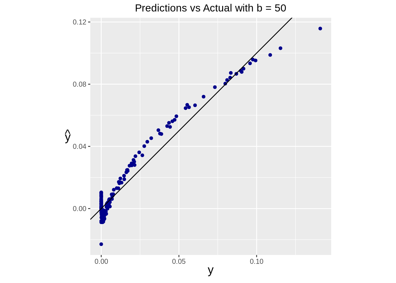
Similarly, we can see the performance of our prediction using the pseudoinverse
ggplot(data=df) +
  geom_point(aes(x=real, y=pseudo_pred), color="darkblue") +
  geom_abline(intercept=0, slope=1) +
  ggtitle(paste("Pseudo-Predictions vs Actual with b =", b)) +
  theme(
    plot.title = element_text(hjust = 0.5),
    axis.title = element_text(size=15, face="bold"),
    axis.title.y = element_text(angle=0, vjust=0.5)
  ) +
  xlab(expression(y)) +
  ylab(expression(hat(y))) +
  coord_fixed()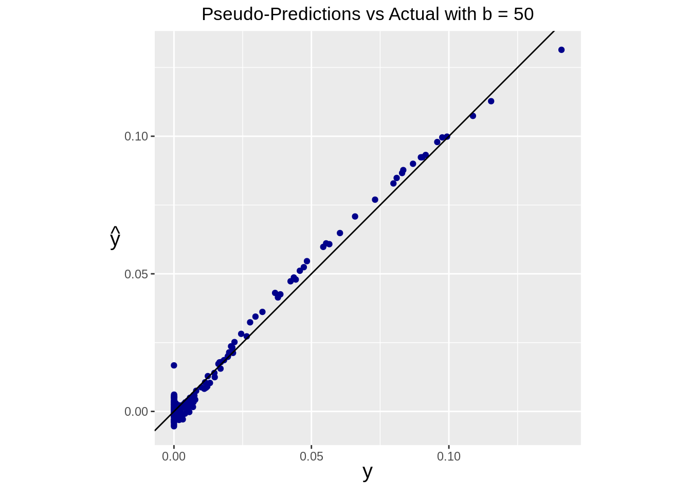
Technical Note on Calculating the Bandwidth
To vectorize this operation, we aim to create a matrix containing all the squared norms of the difference between the vectors \[ D = \begin{pmatrix} \parallel \boldsymbol{\mathbf{x}}_1 - \boldsymbol{\mathbf{x}}_1 \parallel^2 & \parallel \boldsymbol{\mathbf{x}}_1 - \boldsymbol{\mathbf{x}}_2 \parallel^2 & \cdots & \parallel \boldsymbol{\mathbf{x}}_1 - \boldsymbol{\mathbf{x}}_n \parallel^2 \\ \parallel \boldsymbol{\mathbf{x}}_2 - \boldsymbol{\mathbf{x}}_1 \parallel^2 & \parallel \boldsymbol{\mathbf{x}}_2 - \boldsymbol{\mathbf{x}}_2 \parallel^2 & \cdots & \parallel \boldsymbol{\mathbf{x}}_2 - \boldsymbol{\mathbf{x}}_n \parallel^2 \\ \vdots & \vdots & \ddots & \vdots \\ \parallel \boldsymbol{\mathbf{x}}_n - \boldsymbol{\mathbf{x}}_1 \parallel^2 & \parallel \boldsymbol{\mathbf{x}}_n - \boldsymbol{\mathbf{x}}_2 \parallel^2 & \cdots & \parallel \boldsymbol{\mathbf{x}}_n - \boldsymbol{\mathbf{x}}_n \parallel^2 \end{pmatrix} \] Notice that we can rewrite the norm of the difference between two vectors \(\boldsymbol{\mathbf{x}}_i\) and \(\boldsymbol{\mathbf{x}}_j\) as follows \[ \parallel \boldsymbol{\mathbf{x}}_i - \boldsymbol{\mathbf{x}}_j \parallel^2 = (\boldsymbol{\mathbf{x}}_i - \boldsymbol{\mathbf{x}}_j)^\top (\boldsymbol{\mathbf{x}}_i - \boldsymbol{\mathbf{x}}_j) = \boldsymbol{\mathbf{x}}_i^\top\boldsymbol{\mathbf{x}}_i - 2\boldsymbol{\mathbf{x}}_i^\top \boldsymbol{\mathbf{x}}_j + \boldsymbol{\mathbf{x}}_j^\top\boldsymbol{\mathbf{x}}_j \] Broadcasting this, we can rewrite the matrix \(D\) as \[ D = \begin{pmatrix} \boldsymbol{\mathbf{x}}_{1}^\top\boldsymbol{\mathbf{x}}_{1} - 2\boldsymbol{\mathbf{x}}_{1}^\top \boldsymbol{\mathbf{x}}_{1} + \boldsymbol{\mathbf{x}}_{1}^\top\boldsymbol{\mathbf{x}}_{1} & \quad\boldsymbol{\mathbf{x}}_{1}^\top\boldsymbol{\mathbf{x}}_{1} - 2\boldsymbol{\mathbf{x}}_{1}^\top \boldsymbol{\mathbf{x}}_{2} + \boldsymbol{\mathbf{x}}_{2}^\top\boldsymbol{\mathbf{x}}_{2} & \quad\cdots & \quad\boldsymbol{\mathbf{x}}_{1}^\top\boldsymbol{\mathbf{x}}_{1} - 2\boldsymbol{\mathbf{x}}_{1}^\top \boldsymbol{\mathbf{x}}_{n} + \boldsymbol{\mathbf{x}}_{n}^\top\boldsymbol{\mathbf{x}}_{n}\\ \boldsymbol{\mathbf{x}}_{2}^\top\boldsymbol{\mathbf{x}}_{2} - 2\boldsymbol{\mathbf{x}}_{2}^\top \boldsymbol{\mathbf{x}}_{1} + \boldsymbol{\mathbf{x}}_{1}^\top\boldsymbol{\mathbf{x}}_{1} & \quad\boldsymbol{\mathbf{x}}_{2}^\top\boldsymbol{\mathbf{x}}_{2} - 2\boldsymbol{\mathbf{x}}_{2}^\top \boldsymbol{\mathbf{x}}_{2} + \boldsymbol{\mathbf{x}}_{2}^\top\boldsymbol{\mathbf{x}}_{2} & \quad\cdots & \quad\boldsymbol{\mathbf{x}}_{2}^\top\boldsymbol{\mathbf{x}}_{2} - 2\boldsymbol{\mathbf{x}}_{2}^\top \boldsymbol{\mathbf{x}}_{n} + \boldsymbol{\mathbf{x}}_{n}^\top\boldsymbol{\mathbf{x}}_{n}\\ \vdots & \quad\vdots & \quad\ddots & \quad\vdots \\ \boldsymbol{\mathbf{x}}_{n}^\top\boldsymbol{\mathbf{x}}_{n} - 2\boldsymbol{\mathbf{x}}_{n}^\top \boldsymbol{\mathbf{x}}_{1} + \boldsymbol{\mathbf{x}}_{1}^\top\boldsymbol{\mathbf{x}}_{1} & \quad\boldsymbol{\mathbf{x}}_{n}^\top\boldsymbol{\mathbf{x}}_{n} - 2\boldsymbol{\mathbf{x}}_{n}^\top \boldsymbol{\mathbf{x}}_{2} + \boldsymbol{\mathbf{x}}_{2}^\top\boldsymbol{\mathbf{x}}_{2} & \quad\cdots & \quad\boldsymbol{\mathbf{x}}_{n}^\top\boldsymbol{\mathbf{x}}_{n} - 2\boldsymbol{\mathbf{x}}_{n}^\top \boldsymbol{\mathbf{x}}_{n} + \boldsymbol{\mathbf{x}}_{n}^\top\boldsymbol{\mathbf{x}}_{n} \end{pmatrix} \] This can now be split into three matrices, where we can notice that the third matrix is nothing but the transpose of the first. \[ D = \begin{pmatrix} \boldsymbol{\mathbf{x}}_1^\top\boldsymbol{\mathbf{x}}_1 & \boldsymbol{\mathbf{x}}_1^\top\boldsymbol{\mathbf{x}}_1 & \cdots & \boldsymbol{\mathbf{x}}_1^\top\boldsymbol{\mathbf{x}}_1\\ \boldsymbol{\mathbf{x}}_2^\top\boldsymbol{\mathbf{x}}_2 & \boldsymbol{\mathbf{x}}_2^\top\boldsymbol{\mathbf{x}}_2 & \cdots & \boldsymbol{\mathbf{x}}_2^\top\boldsymbol{\mathbf{x}}_2 \\ \vdots & \vdots & \ddots & \vdots\\ \boldsymbol{\mathbf{x}}_n^\top\boldsymbol{\mathbf{x}}_n & \boldsymbol{\mathbf{x}}_n^\top\boldsymbol{\mathbf{x}}_n & \cdots & \boldsymbol{\mathbf{x}}_n^\top\boldsymbol{\mathbf{x}}_n \end{pmatrix} -2 \begin{pmatrix} \boldsymbol{\mathbf{x}}_{1}^\top\boldsymbol{\mathbf{x}}_{1} & \boldsymbol{\mathbf{x}}_{1}^\top\boldsymbol{\mathbf{x}}_{2} & \cdots & \boldsymbol{\mathbf{x}}_{1}^\top\boldsymbol{\mathbf{x}}_{n} \\ \boldsymbol{\mathbf{x}}_{2}^\top\boldsymbol{\mathbf{x}}_{1} & \boldsymbol{\mathbf{x}}_{2}^\top\boldsymbol{\mathbf{x}}_{2} & \cdots & \boldsymbol{\mathbf{x}}_{2}^\top\boldsymbol{\mathbf{x}}_{n} \\ \vdots & \vdots & \ddots & \vdots \\ \boldsymbol{\mathbf{x}}_{n}^\top\boldsymbol{\mathbf{x}}_{1} & \boldsymbol{\mathbf{x}}_{n}^\top\boldsymbol{\mathbf{x}}_{2} & \cdots & \boldsymbol{\mathbf{x}}_{n}^\top\boldsymbol{\mathbf{x}}_{n} \end{pmatrix} + \begin{pmatrix} \boldsymbol{\mathbf{x}}_{1}^\top\boldsymbol{\mathbf{x}}_{1} & \boldsymbol{\mathbf{x}}_{2}^\top\boldsymbol{\mathbf{x}}_{2} & \cdots & \boldsymbol{\mathbf{x}}_{n}^\top\boldsymbol{\mathbf{x}}_{n} \\ \boldsymbol{\mathbf{x}}_{1}^\top\boldsymbol{\mathbf{x}}_{1} & \boldsymbol{\mathbf{x}}_{2}^\top\boldsymbol{\mathbf{x}}_{2} & \cdots & \boldsymbol{\mathbf{x}}_{n}^\top\boldsymbol{\mathbf{x}}_{n} \\ \vdots & \vdots & \ddots & \vdots \\ \boldsymbol{\mathbf{x}}_{1}^\top\boldsymbol{\mathbf{x}}_{1} & \boldsymbol{\mathbf{x}}_{2}^\top\boldsymbol{\mathbf{x}}_{2} & \cdots & \boldsymbol{\mathbf{x}}_{n}^\top\boldsymbol{\mathbf{x}}_{n} \end{pmatrix} \]
The key is not to notice that we can obtain the middle matrix from \(X\) with a simple operation: \[ XX^\top = \begin{pmatrix} \boldsymbol{\mathbf{x}}_1^\top \\ \boldsymbol{\mathbf{x}}_2^\top \\ \vdots \\ \boldsymbol{\mathbf{x}}_n^\top \end{pmatrix} \begin{pmatrix} \boldsymbol{\mathbf{x}}_1 & \boldsymbol{\mathbf{x}}_2 & \cdots & \boldsymbol{\mathbf{x}}_n \end{pmatrix} = \begin{pmatrix} \boldsymbol{\mathbf{x}}_{1}^\top\boldsymbol{\mathbf{x}}_{1} & \boldsymbol{\mathbf{x}}_{1}^\top\boldsymbol{\mathbf{x}}_{2} & \cdots & \boldsymbol{\mathbf{x}}_{1}^\top\boldsymbol{\mathbf{x}}_{n} \\ \boldsymbol{\mathbf{x}}_{2}^\top\boldsymbol{\mathbf{x}}_{1} & \boldsymbol{\mathbf{x}}_{2}^\top\boldsymbol{\mathbf{x}}_{2} & \cdots & \boldsymbol{\mathbf{x}}_{2}^\top\boldsymbol{\mathbf{x}}_{n} \\ \vdots & \vdots & \ddots & \vdots \\ \boldsymbol{\mathbf{x}}_{n}^\top\boldsymbol{\mathbf{x}}_{1} & \boldsymbol{\mathbf{x}}_{n}^\top\boldsymbol{\mathbf{x}}_{2} & \cdots & \boldsymbol{\mathbf{x}}_{n}^\top\boldsymbol{\mathbf{x}}_{n} \end{pmatrix} \]
and then the first matrix can be obtained as follows \[ \begin{pmatrix} 1 \\ 1 \\ \vdots \\ 1 \end{pmatrix}_{n\times 1} \begin{pmatrix} \boldsymbol{\mathbf{x}}_{1}^\top\boldsymbol{\mathbf{x}}_{1} & \boldsymbol{\mathbf{x}}_{2}^\top\boldsymbol{\mathbf{x}}_{2} & \cdots & \boldsymbol{\mathbf{x}}_{n}^\top\boldsymbol{\mathbf{x}}_{n} \end{pmatrix}_{1\times n} = \begin{pmatrix} \boldsymbol{\mathbf{x}}_1^\top\boldsymbol{\mathbf{x}}_1 & \boldsymbol{\mathbf{x}}_1^\top\boldsymbol{\mathbf{x}}_1 & \cdots & \boldsymbol{\mathbf{x}}_1^\top\boldsymbol{\mathbf{x}}_1\\ \boldsymbol{\mathbf{x}}_2^\top\boldsymbol{\mathbf{x}}_2 & \boldsymbol{\mathbf{x}}_2^\top\boldsymbol{\mathbf{x}}_2 & \cdots & \boldsymbol{\mathbf{x}}_2^\top\boldsymbol{\mathbf{x}}_2 \\ \vdots & \vdots & \ddots & \vdots\\ \boldsymbol{\mathbf{x}}_n^\top\boldsymbol{\mathbf{x}}_n & \boldsymbol{\mathbf{x}}_n^\top\boldsymbol{\mathbf{x}}_n & \cdots & \boldsymbol{\mathbf{x}}_n^\top\boldsymbol{\mathbf{x}}_n \end{pmatrix} \] where \[ \text{diag}\left[ \begin{pmatrix} \boldsymbol{\mathbf{x}}_{1}^\top\boldsymbol{\mathbf{x}}_{1} & \boldsymbol{\mathbf{x}}_{1}^\top\boldsymbol{\mathbf{x}}_{2} & \cdots & \boldsymbol{\mathbf{x}}_{1}^\top\boldsymbol{\mathbf{x}}_{n} \\ \boldsymbol{\mathbf{x}}_{2}^\top\boldsymbol{\mathbf{x}}_{1} & \boldsymbol{\mathbf{x}}_{2}^\top\boldsymbol{\mathbf{x}}_{2} & \cdots & \boldsymbol{\mathbf{x}}_{2}^\top\boldsymbol{\mathbf{x}}_{n} \\ \vdots & \vdots & \ddots & \vdots \\ \boldsymbol{\mathbf{x}}_{n}^\top\boldsymbol{\mathbf{x}}_{1} & \boldsymbol{\mathbf{x}}_{n}^\top\boldsymbol{\mathbf{x}}_{2} & \cdots & \boldsymbol{\mathbf{x}}_{n}^\top\boldsymbol{\mathbf{x}}_{n} \end{pmatrix} \right] = \begin{pmatrix} \boldsymbol{\mathbf{x}}_{1}^\top\boldsymbol{\mathbf{x}}_{1} & \boldsymbol{\mathbf{x}}_{2}^\top\boldsymbol{\mathbf{x}}_{2} & \cdots & \boldsymbol{\mathbf{x}}_{n}^\top\boldsymbol{\mathbf{x}}_{n} \end{pmatrix}_{1\times n} \]